注意
点击 这里 下载完整示例代码
TorchVision 物体检测微调教程
创建日期: 2023年12月14日 | 最后更新日期: 2024年6月11日 | 最后验证日期: 2024年11月5日
对于本教程,我们将对预训练的 Mask R-CNN 模型进行微调,使用的是 Penn-Fudan 行人检测和分割数据库。它包含 170 张图像,其中有 345 个行人实例,我们将用它来说明如何使用 torchvision 中的新功能来训练一个自定义数据集的对象检测和实例分割模型。
注意
本教程仅适用于 torchvision 版本 >=0.16 或 nightly 版本。 如果您使用的是 torchvision<=0.15,请参阅 这篇教程。
定义数据集
The reference scripts for training object detection, instance
segmentation and person keypoint detection allows for easily supporting
adding new custom datasets. The dataset should inherit from the standard
torch.utils.data.Dataset 类,并实现 __len__ 和
__getitem__。
我们唯一的要求是数据集 __getitem__
应该返回一个元组:
image:
torchvision.tv_tensors.Image形状为[3, H, W]的张量,或大小为(H, W)的PIL Image目标:一个包含以下字段的字典
boxes,torchvision.tv_tensors.BoundingBoxes形状为[N, 4]:N边界框在[x0, y0, x1, y1]格式下的坐标,范围从0到W和0到Hlabels, 整数torch.Tensor,形状为[N]:每个边界框的标签。0总是表示背景类。image_id, int: 一张图像标识符。在数据集中,它应该是唯一的,并且在评估时使用。area, floattorch.Tensor形状[N]: 边界框的面积。在使用 COCO 指标评估时,此参数用于区分小型、中型和大型边框的度量分数。iscrowd, uint8torch.Tensor形状[N]: 实例具有iscrowd=True将会在评估中被忽略。(optionally)
masks,torchvision.tv_tensors.Mask形状为[N, H, W]:每个对象的分割掩码
如果您的数据集符合上述要求,则可以用于参考脚本中的训练和评估代码。评估代码将使用来自pycocotools的脚本,该脚本可以通过pip install pycocotools安装。
注意
对于Windows,请从gautamchitnis安装pycocotools,使用命令
pip install git+https://github.com/gautamchitnis/cocoapi.git@cocodataset-master#subdirectory=PythonAPI
One note on the labels. The model considers class 0 as background. If your dataset does not contain the background class,
you should not have 0 in your labels. For example, assuming you have just two classes, 猫 and 狗, you can
define 1 (not 0) to represent 猫 and 2 to represent 狗. So, for instance, if one of the images has both
classes, your labels tensor should look like [1, 2].
此外,如果您在训练过程中想要使用方面比组(即每个批次只包含具有相似方面比的图像),则建议也实现一个get_height_and_width
方法,该方法返回图像的高度和宽度。如果没有提供此方法,我们将通过__getitem__ 查询数据集中的所有元素,这将导致图像被加载到内存中,并且速度会慢于提供自定义方法的情况。
编写自定义数据集(PennFudan)
让我们为PennFudan数据集编写一个数据集。首先,让我们下载数据集并解压zip文件:
wget https://www.cis.upenn.edu/~jshi/ped_html/PennFudanPed.zip -P data
cd data && unzip PennFudanPed.zip
我们有以下文件夹结构:
PennFudanPed/
  PedMasks/
    FudanPed00001_mask.png
    FudanPed00002_mask.png
    FudanPed00003_mask.png
    FudanPed00004_mask.png
    ...
  PNGImages/
    FudanPed00001.png
    FudanPed00002.png
    FudanPed00003.png
    FudanPed00004.png
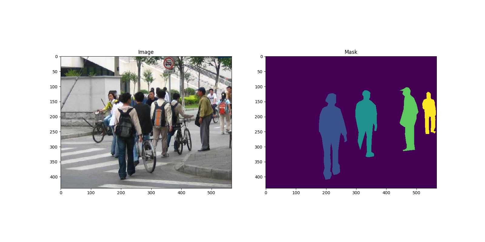
这里有一个图像对的例子,以及相应的分割掩码。
import matplotlib.pyplot as plt
from torchvision.io import read_image


image = read_image("data/PennFudanPed/PNGImages/FudanPed00046.png")
mask = read_image("data/PennFudanPed/PedMasks/FudanPed00046_mask.png")

plt.figure(figsize=(16, 8))
plt.subplot(121)
plt.title("Image")
plt.imshow(image.permute(1, 2, 0))
plt.subplot(122)
plt.title("Mask")
plt.imshow(mask.permute(1, 2, 0))
<matplotlib.image.AxesImage object at 0x7f4edba7ae30>
所以每张图片都有一个对应的分割掩码,其中每种颜色对应一个不同的实例。
让我们为这个数据集编写一个 torch.utils.data.Dataset 类。
在下面的代码中,我们将图片、边界框和掩码包装成 torchvision.tv_tensors.TVTensor 类,以便能够应用 torchvision 内置的转换 (新的 Transforms API)
来完成给定的目标检测和分割任务。
具体来说,图片张量将被包装成 torchvision.tv_tensors.Image,边界框被包装成 torchvision.tv_tensors.BoundingBoxes,掩码被包装成 torchvision.tv_tensors.Mask。
由于 torchvision.tv_tensors.TVTensor 是 torch.Tensor 的子类,因此包装的对象也是张量,并继承了原始的
torch.Tensor API。有关 torchvision tv_tensors 的更多信息,请参阅
此文档。
import os
import torch

from torchvision.io import read_image
from torchvision.ops.boxes import masks_to_boxes
from torchvision import tv_tensors
from torchvision.transforms.v2 import functional as F


class PennFudanDataset(torch.utils.data.Dataset):
    def __init__(self, root, transforms):
        self.root = root
        self.transforms = transforms
        # load all image files, sorting them to
        # ensure that they are aligned
        self.imgs = list(sorted(os.listdir(os.path.join(root, "PNGImages"))))
        self.masks = list(sorted(os.listdir(os.path.join(root, "PedMasks"))))

    def __getitem__(self, idx):
        # load images and masks
        img_path = os.path.join(self.root, "PNGImages", self.imgs[idx])
        mask_path = os.path.join(self.root, "PedMasks", self.masks[idx])
        img = read_image(img_path)
        mask = read_image(mask_path)
        # instances are encoded as different colors
        obj_ids = torch.unique(mask)
        # first id is the background, so remove it
        obj_ids = obj_ids[1:]
        num_objs = len(obj_ids)

        # split the color-encoded mask into a set
        # of binary masks
        masks = (mask == obj_ids[:, None, None]).to(dtype=torch.uint8)

        # get bounding box coordinates for each mask
        boxes = masks_to_boxes(masks)

        # there is only one class
        labels = torch.ones((num_objs,), dtype=torch.int64)

        image_id = idx
        area = (boxes[:, 3] - boxes[:, 1]) * (boxes[:, 2] - boxes[:, 0])
        # suppose all instances are not crowd
        iscrowd = torch.zeros((num_objs,), dtype=torch.int64)

        # Wrap sample and targets into torchvision tv_tensors:
        img = tv_tensors.Image(img)

        target = {}
        target["boxes"] = tv_tensors.BoundingBoxes(boxes, format="XYXY", canvas_size=F.get_size(img))
        target["masks"] = tv_tensors.Mask(masks)
        target["labels"] = labels
        target["image_id"] = image_id
        target["area"] = area
        target["iscrowd"] = iscrowd

        if self.transforms is not None:
            img, target = self.transforms(img, target)

        return img, target

    def __len__(self):
        return len(self.imgs)
这就是关于数据集的所有内容了。现在让我们定义一个模型,这个模型可以在该数据集上进行预测。
定义您的模型
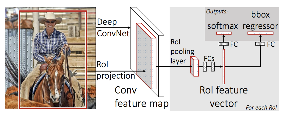
在本教程中,我们将使用 Mask R-CNN,该模型基于 Faster R-CNN。Faster R-CNN 是一种预测图像中潜在对象的边界框和类别得分的模型。
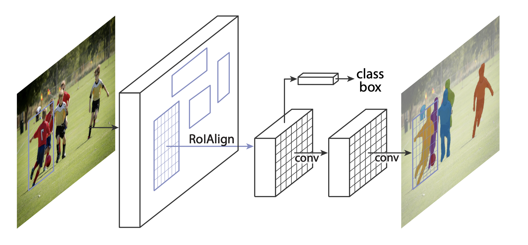
Mask R-CNN 在 Faster R-CNN 的基础上增加了一个额外分支,该分支还预测每个实例的分割掩码。
在 TorchVision Model Zoo中,有两类常见的场景需要修改已有的模型。第一类是当我们希望从一个预训练模型开始,并仅微调最后一层。另一类是当我们想用不同的骨干网络替换当前模型的骨干网络(例如为了更快的预测)。
让我们在接下来的部分看看我们是如何实现其中的一种或另一种的。
1 - 从预训练模型微调
假设你想从一个在 COCO 数据集上预训练好的模型开始,并希望对其进行微调以适应你特定的类别。这里是一种可能的方法:
import torchvision
from torchvision.models.detection.faster_rcnn import FastRCNNPredictor

# load a model pre-trained on COCO
model = torchvision.models.detection.fasterrcnn_resnet50_fpn(weights="DEFAULT")

# replace the classifier with a new one, that has
# num_classes which is user-defined
num_classes = 2  # 1 class (person) + background
# get number of input features for the classifier
in_features = model.roi_heads.box_predictor.cls_score.in_features
# replace the pre-trained head with a new one
model.roi_heads.box_predictor = FastRCNNPredictor(in_features, num_classes)
Downloading: "https://download.pytorch.org/models/fasterrcnn_resnet50_fpn_coco-258fb6c6.pth" to /var/lib/ci-user/.cache/torch/hub/checkpoints/fasterrcnn_resnet50_fpn_coco-258fb6c6.pth

  0%|          | 0.00/160M [00:00<?, ?B/s]
 27%|##6       | 42.8M/160M [00:00<00:00, 448MB/s]
 54%|#####4    | 86.8M/160M [00:00<00:00, 456MB/s]
 82%|########1 | 131M/160M [00:00<00:00, 458MB/s]
100%|##########| 160M/160M [00:00<00:00, 457MB/s]
2 - 修改模型以添加不同的骨干网络
import torchvision
from torchvision.models.detection import FasterRCNN
from torchvision.models.detection.rpn import AnchorGenerator

# load a pre-trained model for classification and return
# only the features
backbone = torchvision.models.mobilenet_v2(weights="DEFAULT").features
# ``FasterRCNN`` needs to know the number of
# output channels in a backbone. For mobilenet_v2, it's 1280
# so we need to add it here
backbone.out_channels = 1280

# let's make the RPN generate 5 x 3 anchors per spatial
# location, with 5 different sizes and 3 different aspect
# ratios. We have a Tuple[Tuple[int]] because each feature
# map could potentially have different sizes and
# aspect ratios
anchor_generator = AnchorGenerator(
    sizes=((32, 64, 128, 256, 512),),
    aspect_ratios=((0.5, 1.0, 2.0),)
)

# let's define what are the feature maps that we will
# use to perform the region of interest cropping, as well as
# the size of the crop after rescaling.
# if your backbone returns a Tensor, featmap_names is expected to
# be [0]. More generally, the backbone should return an
# ``OrderedDict[Tensor]``, and in ``featmap_names`` you can choose which
# feature maps to use.
roi_pooler = torchvision.ops.MultiScaleRoIAlign(
    featmap_names=['0'],
    output_size=7,
    sampling_ratio=2
)

# put the pieces together inside a Faster-RCNN model
model = FasterRCNN(
    backbone,
    num_classes=2,
    rpn_anchor_generator=anchor_generator,
    box_roi_pool=roi_pooler
)
Downloading: "https://download.pytorch.org/models/mobilenet_v2-7ebf99e0.pth" to /var/lib/ci-user/.cache/torch/hub/checkpoints/mobilenet_v2-7ebf99e0.pth

  0%|          | 0.00/13.6M [00:00<?, ?B/s]
100%|##########| 13.6M/13.6M [00:00<00:00, 381MB/s]
PennFudan 数据集的对象检测和实例分割模型
在我们的情况下,由于数据集非常小,我们希望从一个预训练模型进行微调,因此我们将遵循方法一。
在这里,我们还想计算实例分割掩码,因此我们将使用Mask R-CNN:
import torchvision
from torchvision.models.detection.faster_rcnn import FastRCNNPredictor
from torchvision.models.detection.mask_rcnn import MaskRCNNPredictor


def get_model_instance_segmentation(num_classes):
    # load an instance segmentation model pre-trained on COCO
    model = torchvision.models.detection.maskrcnn_resnet50_fpn(weights="DEFAULT")

    # get number of input features for the classifier
    in_features = model.roi_heads.box_predictor.cls_score.in_features
    # replace the pre-trained head with a new one
    model.roi_heads.box_predictor = FastRCNNPredictor(in_features, num_classes)

    # now get the number of input features for the mask classifier
    in_features_mask = model.roi_heads.mask_predictor.conv5_mask.in_channels
    hidden_layer = 256
    # and replace the mask predictor with a new one
    model.roi_heads.mask_predictor = MaskRCNNPredictor(
        in_features_mask,
        hidden_layer,
        num_classes
    )

    return model
这就是全部,这将使 model 可以在您自定义的数据集上进行训练和评估。
Putting everything together
在 references/detection/ 中,我们提供了一系列辅助函数来简化检测模型的训练和评估过程。这里,我们将使用 references/detection/engine.py 和 references/detection/utils.py。
只需将 references/detection 下方的所有内容下载到您的文件夹并在此处使用。
在 Linux 系统上,如果您有 wget,可以使用以下命令下载它们:
os.system("wget https://raw.githubusercontent.com/pytorch/vision/main/references/detection/engine.py")
os.system("wget https://raw.githubusercontent.com/pytorch/vision/main/references/detection/utils.py")
os.system("wget https://raw.githubusercontent.com/pytorch/vision/main/references/detection/coco_utils.py")
os.system("wget https://raw.githubusercontent.com/pytorch/vision/main/references/detection/coco_eval.py")
os.system("wget https://raw.githubusercontent.com/pytorch/vision/main/references/detection/transforms.py")
0
自 v0.15.0 版本以来,torchvision 提供了 新的 Transforms API ,可以轻松编写用于目标检测和分割任务的数据增强管道。
让我们编写一些辅助函数来进行数据增强/转换:
from torchvision.transforms import v2 as T


def get_transform(train):
    transforms = []
    if train:
        transforms.append(T.RandomHorizontalFlip(0.5))
    transforms.append(T.ToDtype(torch.float, scale=True))
    transforms.append(T.ToPureTensor())
    return T.Compose(transforms)
测试 forward() 方法(可选)
在遍历数据集之前,最好查看一下模型在训练和推理过程中对样本数据的期望。
import utils

model = torchvision.models.detection.fasterrcnn_resnet50_fpn(weights="DEFAULT")
dataset = PennFudanDataset('data/PennFudanPed', get_transform(train=True))
data_loader = torch.utils.data.DataLoader(
    dataset,
    batch_size=2,
    shuffle=True,
    collate_fn=utils.collate_fn
)

# For Training
images, targets = next(iter(data_loader))
images = list(image for image in images)
targets = [{k: v for k, v in t.items()} for t in targets]
output = model(images, targets)  # Returns losses and detections
print(output)

# For inference
model.eval()
x = [torch.rand(3, 300, 400), torch.rand(3, 500, 400)]
predictions = model(x)  # Returns predictions
print(predictions[0])
{'loss_classifier': tensor(0.0808, grad_fn=<NllLossBackward0>), 'loss_box_reg': tensor(0.0284, grad_fn=<DivBackward0>), 'loss_objectness': tensor(0.0186, grad_fn=<BinaryCrossEntropyWithLogitsBackward0>), 'loss_rpn_box_reg': tensor(0.0034, grad_fn=<DivBackward0>)}
{'boxes': tensor([], size=(0, 4), grad_fn=<StackBackward0>), 'labels': tensor([], dtype=torch.int64), 'scores': tensor([], grad_fn=<IndexBackward0>)}
现在让我们编写主要函数,该函数执行训练和验证:
from engine import train_one_epoch, evaluate

# train on the GPU or on the CPU, if a GPU is not available
device = torch.device('cuda') if torch.cuda.is_available() else torch.device('cpu')

# our dataset has two classes only - background and person
num_classes = 2
# use our dataset and defined transformations
dataset = PennFudanDataset('data/PennFudanPed', get_transform(train=True))
dataset_test = PennFudanDataset('data/PennFudanPed', get_transform(train=False))

# split the dataset in train and test set
indices = torch.randperm(len(dataset)).tolist()
dataset = torch.utils.data.Subset(dataset, indices[:-50])
dataset_test = torch.utils.data.Subset(dataset_test, indices[-50:])

# define training and validation data loaders
data_loader = torch.utils.data.DataLoader(
    dataset,
    batch_size=2,
    shuffle=True,
    collate_fn=utils.collate_fn
)

data_loader_test = torch.utils.data.DataLoader(
    dataset_test,
    batch_size=1,
    shuffle=False,
    collate_fn=utils.collate_fn
)

# get the model using our helper function
model = get_model_instance_segmentation(num_classes)

# move model to the right device
model.to(device)

# construct an optimizer
params = [p for p in model.parameters() if p.requires_grad]
optimizer = torch.optim.SGD(
    params,
    lr=0.005,
    momentum=0.9,
    weight_decay=0.0005
)

# and a learning rate scheduler
lr_scheduler = torch.optim.lr_scheduler.StepLR(
    optimizer,
    step_size=3,
    gamma=0.1
)

# let's train it just for 2 epochs
num_epochs = 2

for epoch in range(num_epochs):
    # train for one epoch, printing every 10 iterations
    train_one_epoch(model, optimizer, data_loader, device, epoch, print_freq=10)
    # update the learning rate
    lr_scheduler.step()
    # evaluate on the test dataset
    evaluate(model, data_loader_test, device=device)

print("That's it!")
Downloading: "https://download.pytorch.org/models/maskrcnn_resnet50_fpn_coco-bf2d0c1e.pth" to /var/lib/ci-user/.cache/torch/hub/checkpoints/maskrcnn_resnet50_fpn_coco-bf2d0c1e.pth

  0%|          | 0.00/170M [00:00<?, ?B/s]
 25%|##5       | 42.8M/170M [00:00<00:00, 448MB/s]
 52%|#####1    | 87.5M/170M [00:00<00:00, 460MB/s]
 78%|#######7  | 132M/170M [00:00<00:00, 463MB/s]
100%|##########| 170M/170M [00:00<00:00, 462MB/s]
/var/lib/workspace/intermediate_source/engine.py:30: FutureWarning:

`torch.cuda.amp.autocast(args...)` is deprecated. Please use `torch.amp.autocast('cuda', args...)` instead.

Epoch: [0]  [ 0/60]  eta: 0:00:23  lr: 0.000090  loss: 4.9024 (4.9024)  loss_classifier: 0.4325 (0.4325)  loss_box_reg: 0.1060 (0.1060)  loss_mask: 4.3588 (4.3588)  loss_objectness: 0.0028 (0.0028)  loss_rpn_box_reg: 0.0023 (0.0023)  time: 0.3958  data: 0.0135  max mem: 2430
Epoch: [0]  [10/60]  eta: 0:00:11  lr: 0.000936  loss: 1.7743 (2.7696)  loss_classifier: 0.4134 (0.3553)  loss_box_reg: 0.3051 (0.2540)  loss_mask: 0.9491 (2.1320)  loss_objectness: 0.0218 (0.0214)  loss_rpn_box_reg: 0.0056 (0.0069)  time: 0.2267  data: 0.0151  max mem: 2594
Epoch: [0]  [20/60]  eta: 0:00:08  lr: 0.001783  loss: 0.8078 (1.7882)  loss_classifier: 0.2145 (0.2678)  loss_box_reg: 0.2062 (0.2328)  loss_mask: 0.3990 (1.2594)  loss_objectness: 0.0134 (0.0202)  loss_rpn_box_reg: 0.0076 (0.0080)  time: 0.2064  data: 0.0154  max mem: 2628
Epoch: [0]  [30/60]  eta: 0:00:06  lr: 0.002629  loss: 0.6568 (1.4240)  loss_classifier: 0.1409 (0.2251)  loss_box_reg: 0.2294 (0.2425)  loss_mask: 0.2605 (0.9280)  loss_objectness: 0.0122 (0.0186)  loss_rpn_box_reg: 0.0101 (0.0099)  time: 0.2106  data: 0.0163  max mem: 2772
Epoch: [0]  [40/60]  eta: 0:00:04  lr: 0.003476  loss: 0.5629 (1.2055)  loss_classifier: 0.0928 (0.1906)  loss_box_reg: 0.2512 (0.2357)  loss_mask: 0.2267 (0.7537)  loss_objectness: 0.0076 (0.0156)  loss_rpn_box_reg: 0.0119 (0.0098)  time: 0.2101  data: 0.0167  max mem: 2772
Epoch: [0]  [50/60]  eta: 0:00:02  lr: 0.004323  loss: 0.3608 (1.0399)  loss_classifier: 0.0590 (0.1624)  loss_box_reg: 0.1578 (0.2174)  loss_mask: 0.1602 (0.6378)  loss_objectness: 0.0019 (0.0130)  loss_rpn_box_reg: 0.0071 (0.0093)  time: 0.2051  data: 0.0161  max mem: 2772
Epoch: [0]  [59/60]  eta: 0:00:00  lr: 0.005000  loss: 0.3463 (0.9410)  loss_classifier: 0.0383 (0.1445)  loss_box_reg: 0.1258 (0.2049)  loss_mask: 0.1596 (0.5712)  loss_objectness: 0.0015 (0.0115)  loss_rpn_box_reg: 0.0064 (0.0089)  time: 0.2012  data: 0.0153  max mem: 2772
Epoch: [0] Total time: 0:00:12 (0.2094 s / it)
creating index...
index created!
Test:  [ 0/50]  eta: 0:00:04  model_time: 0.0785 (0.0785)  evaluator_time: 0.0074 (0.0074)  time: 0.0988  data: 0.0124  max mem: 2772
Test:  [49/50]  eta: 0:00:00  model_time: 0.0420 (0.0571)  evaluator_time: 0.0049 (0.0072)  time: 0.0641  data: 0.0097  max mem: 2772
Test: Total time: 0:00:03 (0.0755 s / it)
Averaged stats: model_time: 0.0420 (0.0571)  evaluator_time: 0.0049 (0.0072)
Accumulating evaluation results...
DONE (t=0.01s).
Accumulating evaluation results...
DONE (t=0.01s).
IoU metric: bbox
 Average Precision  (AP) @[ IoU=0.50:0.95 | area=   all | maxDets=100 ] = 0.645
 Average Precision  (AP) @[ IoU=0.50      | area=   all | maxDets=100 ] = 0.984
 Average Precision  (AP) @[ IoU=0.75      | area=   all | maxDets=100 ] = 0.854
 Average Precision  (AP) @[ IoU=0.50:0.95 | area= small | maxDets=100 ] = 0.288
 Average Precision  (AP) @[ IoU=0.50:0.95 | area=medium | maxDets=100 ] = 0.622
 Average Precision  (AP) @[ IoU=0.50:0.95 | area= large | maxDets=100 ] = 0.657
 Average Recall     (AR) @[ IoU=0.50:0.95 | area=   all | maxDets=  1 ] = 0.282
 Average Recall     (AR) @[ IoU=0.50:0.95 | area=   all | maxDets= 10 ] = 0.699
 Average Recall     (AR) @[ IoU=0.50:0.95 | area=   all | maxDets=100 ] = 0.699
 Average Recall     (AR) @[ IoU=0.50:0.95 | area= small | maxDets=100 ] = 0.367
 Average Recall     (AR) @[ IoU=0.50:0.95 | area=medium | maxDets=100 ] = 0.692
 Average Recall     (AR) @[ IoU=0.50:0.95 | area= large | maxDets=100 ] = 0.709
IoU metric: segm
 Average Precision  (AP) @[ IoU=0.50:0.95 | area=   all | maxDets=100 ] = 0.669
 Average Precision  (AP) @[ IoU=0.50      | area=   all | maxDets=100 ] = 0.975
 Average Precision  (AP) @[ IoU=0.75      | area=   all | maxDets=100 ] = 0.793
 Average Precision  (AP) @[ IoU=0.50:0.95 | area= small | maxDets=100 ] = 0.394
 Average Precision  (AP) @[ IoU=0.50:0.95 | area=medium | maxDets=100 ] = 0.517
 Average Precision  (AP) @[ IoU=0.50:0.95 | area= large | maxDets=100 ] = 0.685
 Average Recall     (AR) @[ IoU=0.50:0.95 | area=   all | maxDets=  1 ] = 0.290
 Average Recall     (AR) @[ IoU=0.50:0.95 | area=   all | maxDets= 10 ] = 0.720
 Average Recall     (AR) @[ IoU=0.50:0.95 | area=   all | maxDets=100 ] = 0.724
 Average Recall     (AR) @[ IoU=0.50:0.95 | area= small | maxDets=100 ] = 0.633
 Average Recall     (AR) @[ IoU=0.50:0.95 | area=medium | maxDets=100 ] = 0.658
 Average Recall     (AR) @[ IoU=0.50:0.95 | area= large | maxDets=100 ] = 0.734
Epoch: [1]  [ 0/60]  eta: 0:00:11  lr: 0.005000  loss: 0.2605 (0.2605)  loss_classifier: 0.0164 (0.0164)  loss_box_reg: 0.0640 (0.0640)  loss_mask: 0.1767 (0.1767)  loss_objectness: 0.0001 (0.0001)  loss_rpn_box_reg: 0.0032 (0.0032)  time: 0.1859  data: 0.0200  max mem: 2772
Epoch: [1]  [10/60]  eta: 0:00:10  lr: 0.005000  loss: 0.3323 (0.3736)  loss_classifier: 0.0424 (0.0505)  loss_box_reg: 0.1275 (0.1469)  loss_mask: 0.1594 (0.1662)  loss_objectness: 0.0008 (0.0017)  loss_rpn_box_reg: 0.0077 (0.0082)  time: 0.2085  data: 0.0170  max mem: 2772
Epoch: [1]  [20/60]  eta: 0:00:08  lr: 0.005000  loss: 0.3343 (0.3471)  loss_classifier: 0.0412 (0.0440)  loss_box_reg: 0.1203 (0.1213)  loss_mask: 0.1660 (0.1731)  loss_objectness: 0.0009 (0.0016)  loss_rpn_box_reg: 0.0068 (0.0070)  time: 0.2051  data: 0.0155  max mem: 2772
Epoch: [1]  [30/60]  eta: 0:00:06  lr: 0.005000  loss: 0.3024 (0.3285)  loss_classifier: 0.0358 (0.0442)  loss_box_reg: 0.0852 (0.1143)  loss_mask: 0.1521 (0.1616)  loss_objectness: 0.0009 (0.0015)  loss_rpn_box_reg: 0.0045 (0.0068)  time: 0.2044  data: 0.0155  max mem: 2772
Epoch: [1]  [40/60]  eta: 0:00:04  lr: 0.005000  loss: 0.2724 (0.3243)  loss_classifier: 0.0425 (0.0435)  loss_box_reg: 0.0852 (0.1082)  loss_mask: 0.1456 (0.1638)  loss_objectness: 0.0012 (0.0016)  loss_rpn_box_reg: 0.0051 (0.0071)  time: 0.2043  data: 0.0161  max mem: 2772
Epoch: [1]  [50/60]  eta: 0:00:02  lr: 0.005000  loss: 0.2579 (0.3127)  loss_classifier: 0.0328 (0.0416)  loss_box_reg: 0.0590 (0.1009)  loss_mask: 0.1590 (0.1619)  loss_objectness: 0.0016 (0.0017)  loss_rpn_box_reg: 0.0040 (0.0066)  time: 0.2028  data: 0.0151  max mem: 2772
Epoch: [1]  [59/60]  eta: 0:00:00  lr: 0.005000  loss: 0.2166 (0.2985)  loss_classifier: 0.0293 (0.0406)  loss_box_reg: 0.0522 (0.0942)  loss_mask: 0.1260 (0.1557)  loss_objectness: 0.0008 (0.0016)  loss_rpn_box_reg: 0.0035 (0.0063)  time: 0.2050  data: 0.0157  max mem: 2772
Epoch: [1] Total time: 0:00:12 (0.2046 s / it)
creating index...
index created!
Test:  [ 0/50]  eta: 0:00:02  model_time: 0.0410 (0.0410)  evaluator_time: 0.0038 (0.0038)  time: 0.0579  data: 0.0126  max mem: 2772
Test:  [49/50]  eta: 0:00:00  model_time: 0.0396 (0.0405)  evaluator_time: 0.0030 (0.0040)  time: 0.0544  data: 0.0096  max mem: 2772
Test: Total time: 0:00:02 (0.0556 s / it)
Averaged stats: model_time: 0.0396 (0.0405)  evaluator_time: 0.0030 (0.0040)
Accumulating evaluation results...
DONE (t=0.01s).
Accumulating evaluation results...
DONE (t=0.01s).
IoU metric: bbox
 Average Precision  (AP) @[ IoU=0.50:0.95 | area=   all | maxDets=100 ] = 0.767
 Average Precision  (AP) @[ IoU=0.50      | area=   all | maxDets=100 ] = 0.986
 Average Precision  (AP) @[ IoU=0.75      | area=   all | maxDets=100 ] = 0.933
 Average Precision  (AP) @[ IoU=0.50:0.95 | area= small | maxDets=100 ] = 0.378
 Average Precision  (AP) @[ IoU=0.50:0.95 | area=medium | maxDets=100 ] = 0.702
 Average Precision  (AP) @[ IoU=0.50:0.95 | area= large | maxDets=100 ] = 0.783
 Average Recall     (AR) @[ IoU=0.50:0.95 | area=   all | maxDets=  1 ] = 0.331
 Average Recall     (AR) @[ IoU=0.50:0.95 | area=   all | maxDets= 10 ] = 0.810
 Average Recall     (AR) @[ IoU=0.50:0.95 | area=   all | maxDets=100 ] = 0.810
 Average Recall     (AR) @[ IoU=0.50:0.95 | area= small | maxDets=100 ] = 0.433
 Average Recall     (AR) @[ IoU=0.50:0.95 | area=medium | maxDets=100 ] = 0.792
 Average Recall     (AR) @[ IoU=0.50:0.95 | area= large | maxDets=100 ] = 0.822
IoU metric: segm
 Average Precision  (AP) @[ IoU=0.50:0.95 | area=   all | maxDets=100 ] = 0.731
 Average Precision  (AP) @[ IoU=0.50      | area=   all | maxDets=100 ] = 0.980
 Average Precision  (AP) @[ IoU=0.75      | area=   all | maxDets=100 ] = 0.899
 Average Precision  (AP) @[ IoU=0.50:0.95 | area= small | maxDets=100 ] = 0.421
 Average Precision  (AP) @[ IoU=0.50:0.95 | area=medium | maxDets=100 ] = 0.575
 Average Precision  (AP) @[ IoU=0.50:0.95 | area= large | maxDets=100 ] = 0.749
 Average Recall     (AR) @[ IoU=0.50:0.95 | area=   all | maxDets=  1 ] = 0.319
 Average Recall     (AR) @[ IoU=0.50:0.95 | area=   all | maxDets= 10 ] = 0.777
 Average Recall     (AR) @[ IoU=0.50:0.95 | area=   all | maxDets=100 ] = 0.777
 Average Recall     (AR) @[ IoU=0.50:0.95 | area= small | maxDets=100 ] = 0.533
 Average Recall     (AR) @[ IoU=0.50:0.95 | area=medium | maxDets=100 ] = 0.725
 Average Recall     (AR) @[ IoU=0.50:0.95 | area= large | maxDets=100 ] = 0.789
That's it!
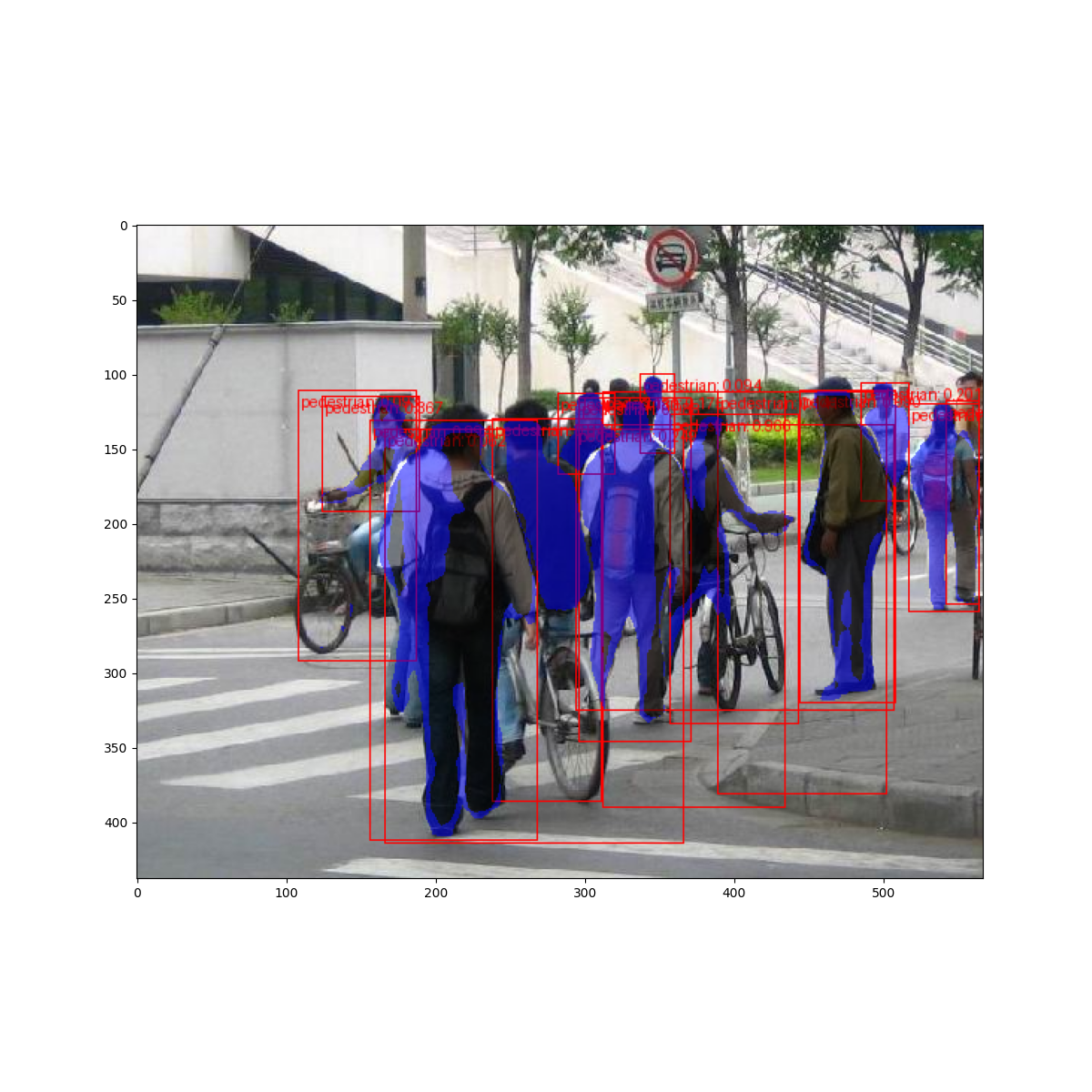
经过一轮训练后,我们得到的mAP超过50%,并且掩码mAP为65%。
但预测结果是什么样的呢?让我们取一个数据集中的图像来验证一下。
import matplotlib.pyplot as plt

from torchvision.utils import draw_bounding_boxes, draw_segmentation_masks


image = read_image("data/PennFudanPed/PNGImages/FudanPed00046.png")
eval_transform = get_transform(train=False)

model.eval()
with torch.no_grad():
    x = eval_transform(image)
    # convert RGBA -> RGB and move to device
    x = x[:3, ...].to(device)
    predictions = model([x, ])
    pred = predictions[0]


image = (255.0 * (image - image.min()) / (image.max() - image.min())).to(torch.uint8)
image = image[:3, ...]
pred_labels = [f"pedestrian: {score:.3f}" for label, score in zip(pred["labels"], pred["scores"])]
pred_boxes = pred["boxes"].long()
output_image = draw_bounding_boxes(image, pred_boxes, pred_labels, colors="red")

masks = (pred["masks"] > 0.7).squeeze(1)
output_image = draw_segmentation_masks(output_image, masks, alpha=0.5, colors="blue")


plt.figure(figsize=(12, 12))
plt.imshow(output_image.permute(1, 2, 0))
<matplotlib.image.AxesImage object at 0x7f4edb52d7b0>
结果看起来很好!
总结
在本教程中,您已经学会了如何为自定义数据集创建自己的对象检测模型训练管道。为此,您编写了一个torch.utils.data.Dataset类,该类返回图像和地面真实框及分割掩码。您还利用了在COCO train2017上预训练的Mask R-CNN模型来进行此新数据集的迁移学习。
对于更完整的示例,其中包括多机/多GPU训练,请参阅references/detection/train.py,该示例位于torchvision仓库中。
脚本总运行时间: ( 0 分钟 46.025 秒)