自定义函数中的双微分

创建日期: 2021年8月13日 | 最后更新日期: 2021年8月13日 | 最后验证日期: 2024年11月5日

有时需要通过反向图运行两次反向传播，例如计算高阶梯度。然而，这需要对自动求导（autograd）有深入的理解，并且需要注意一些细节。支持一次反向传播的函数未必能够支持两次反向传播。在本教程中，我们将展示如何编写一个支持两次反向传播的自定义自动求导函数，并指出一些需要注意的问题。

当编写自定义自动求导函数以便在自定义函数中正向和反向遍历两次时，了解哪些操作在自定义函数中被自动求导记录，哪些不被记录，最重要的是，了解save_for_backward如何与这一切交互。

自定义函数会以两种方式隐式影响梯度模式：

• 在前向传播过程中，autograd 不会在前向函数内执行的任何操作中记录任何计算图。当前向传播完成后，自定义函数的反向传播函数变为每个前向输出的 grad_fn

• 在反向传播过程中，如果指定了`create_graph`，autograd将会记录用于计算反向传播的计算图。

接下来，为了理解 save_for_backward 如何与上述内容交互， 我们可以探索几个示例:

保存输入

考虑这个简单的平方函数。它会保存输入张量以备反向传播时使用。当自动微分能够记录反向传播过程中进行的操作时，双反向传播会自动工作，因此通常不需要担心当我们保存输入张量以备反向传播时的情况，因为只要该输入张量是任何需要梯度的张量的函数，它就应该有 grad_fn，这使得梯度能够正确地传递。

import torch

class Square(torch.autograd.Function):
    @staticmethod
    def forward(ctx, x):
        # Because we are saving one of the inputs use `save_for_backward`
        # Save non-tensors and non-inputs/non-outputs directly on ctx
        ctx.save_for_backward(x)
        return x**2

    @staticmethod
    def backward(ctx, grad_out):
        # A function support double backward automatically if autograd
        # is able to record the computations performed in backward
        x, = ctx.saved_tensors
        return grad_out * 2 * x

# Use double precision because finite differencing method magnifies errors
x = torch.rand(3, 3, requires_grad=True, dtype=torch.double)
torch.autograd.gradcheck(Square.apply, x)
# Use gradcheck to verify second-order derivatives
torch.autograd.gradgradcheck(Square.apply, x)

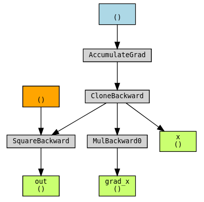
我们可以使用torchviz来可视化图形，以便了解为什么这样做有效。

import torchviz

x = torch.tensor(1., requires_grad=True).clone()
out = Square.apply(x)
grad_x, = torch.autograd.grad(out, x, create_graph=True)
torchviz.make_dot((grad_x, x, out), {"grad_x": grad_x, "x": x, "out": out})

我们可以看到，x 的梯度本身是 x 的一个函数（dout/dx = 2x）。 并且，这个函数的图形已经正确构建。

保存输出

前一个示例稍作变化，可以保存输出而不是输入。由于输出也与 grad_fn 相关联，因此其机械原理是相似的。

class Exp(torch.autograd.Function):
    # Simple case where everything goes well
    @staticmethod
    def forward(ctx, x):
        # This time we save the output
        result = torch.exp(x)
        # Note that we should use `save_for_backward` here when
        # the tensor saved is an ouptut (or an input).
        ctx.save_for_backward(result)
        return result

    @staticmethod
    def backward(ctx, grad_out):
        result, = ctx.saved_tensors
        return result * grad_out

x = torch.tensor(1., requires_grad=True, dtype=torch.double).clone()
# Validate our gradients using gradcheck
torch.autograd.gradcheck(Exp.apply, x)
torch.autograd.gradgradcheck(Exp.apply, x)

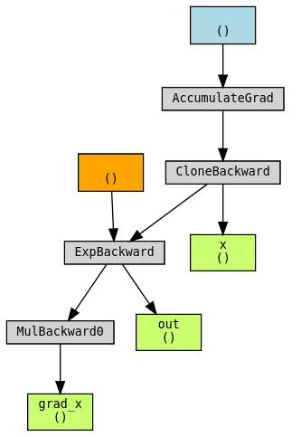
使用 torchviz 来可视化图形：

out = Exp.apply(x)
grad_x, = torch.autograd.grad(out, x, create_graph=True)
torchviz.make_dot((grad_x, x, out), {"grad_x": grad_x, "x": x, "out": out})

保存中间结果

一个更棘手的情况是我们需要保存中间结果。 我们通过实现以下内容来演示这种情形：

\[sinh(x) := \frac{e^x - e^{-x}}{2} \]

由于 sinh 的导数是 cosh，因此在正向传播中计算的两个中间结果 exp(x) 和 exp(-x) 可能在反向传播计算中重用是有用的。

中间结果不应直接保存并在反向传播中使用。 因为前向传播是在无梯度模式下进行的，如果在反向传播中使用了前向传播过程中的中间结果来计算梯度，那么梯度的反向图将不会包括计算中间结果的操作。这会导致梯度不正确。

class Sinh(torch.autograd.Function):
    @staticmethod
    def forward(ctx, x):
        expx = torch.exp(x)
        expnegx = torch.exp(-x)
        ctx.save_for_backward(expx, expnegx)
        # In order to be able to save the intermediate results, a trick is to
        # include them as our outputs, so that the backward graph is constructed
        return (expx - expnegx) / 2, expx, expnegx

    @staticmethod
    def backward(ctx, grad_out, _grad_out_exp, _grad_out_negexp):
        expx, expnegx = ctx.saved_tensors
        grad_input = grad_out * (expx + expnegx) / 2
        # We cannot skip accumulating these even though we won't use the outputs
        # directly. They will be used later in the second backward.
        grad_input += _grad_out_exp * expx
        grad_input -= _grad_out_negexp * expnegx
        return grad_input

def sinh(x):
    # Create a wrapper that only returns the first output
    return Sinh.apply(x)[0]

x = torch.rand(3, 3, requires_grad=True, dtype=torch.double)
torch.autograd.gradcheck(sinh, x)
torch.autograd.gradgradcheck(sinh, x)

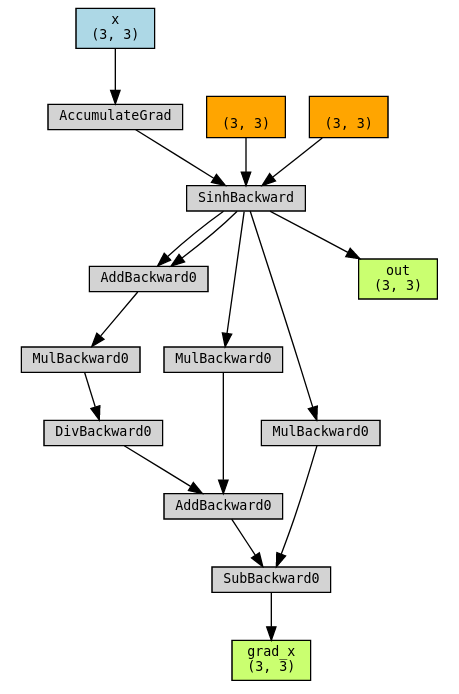
使用 torchviz 来可视化图形：

out = sinh(x)
grad_x, = torch.autograd.grad(out.sum(), x, create_graph=True)
torchviz.make_dot((grad_x, x, out), params={"grad_x": grad_x, "x": x, "out": out})

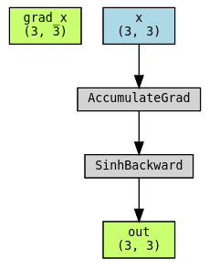
保存中间结果：不该做什么

现在我们展示一下当我们不也将中间结果作为输出返回时会发生什么：grad_x甚至不会有一个反向图，因为它纯粹是函数 exp 和 expnegx 的结果，而这两个函数不需要 grad。

class SinhBad(torch.autograd.Function):
    # This is an example of what NOT to do!
    @staticmethod
    def forward(ctx, x):
        expx = torch.exp(x)
        expnegx = torch.exp(-x)
        ctx.expx = expx
        ctx.expnegx = expnegx
        return (expx - expnegx) / 2

    @staticmethod
    def backward(ctx, grad_out):
        expx = ctx.expx
        expnegx = ctx.expnegx
        grad_input = grad_out * (expx + expnegx) / 2
        return grad_input

使用 torchviz 来可视化图形。请注意，grad_x 不是图形的一部分！

out = SinhBad.apply(x)
grad_x, = torch.autograd.grad(out.sum(), x, create_graph=True)
torchviz.make_dot((grad_x, x, out), params={"grad_x": grad_x, "x": x, "out": out})

当反向传播未被跟踪

最后，让我们考虑一个例子，在这个例子中，autograd 可能无法跟踪 cube_backward 函数反向传播时的梯度。 我们可以想象 cube_backward 是一个可能需要像 SciPy 或 NumPy 这样的非 PyTorch 库，或者是一个用 C++ 扩展编写的函数。这里展示的解决方案是创建另一个自定义函数 CubeBackward，同时手动指定 cube_backward 的反向传播！

def cube_forward(x):
    return x**3

def cube_backward(grad_out, x):
    return grad_out * 3 * x**2

def cube_backward_backward(grad_out, sav_grad_out, x):
    return grad_out * sav_grad_out * 6 * x

def cube_backward_backward_grad_out(grad_out, x):
    return grad_out * 3 * x**2

class Cube(torch.autograd.Function):
    @staticmethod
    def forward(ctx, x):
        ctx.save_for_backward(x)
        return cube_forward(x)

    @staticmethod
    def backward(ctx, grad_out):
        x, = ctx.saved_tensors
        return CubeBackward.apply(grad_out, x)

class CubeBackward(torch.autograd.Function):
    @staticmethod
    def forward(ctx, grad_out, x):
        ctx.save_for_backward(x, grad_out)
        return cube_backward(grad_out, x)

    @staticmethod
    def backward(ctx, grad_out):
        x, sav_grad_out = ctx.saved_tensors
        dx = cube_backward_backward(grad_out, sav_grad_out, x)
        dgrad_out = cube_backward_backward_grad_out(grad_out, x)
        return dgrad_out, dx

x = torch.tensor(2., requires_grad=True, dtype=torch.double)

torch.autograd.gradcheck(Cube.apply, x)
torch.autograd.gradgradcheck(Cube.apply, x)

使用 torchviz 来可视化图形：

out = Cube.apply(x)
grad_x, = torch.autograd.grad(out, x, create_graph=True)
torchviz.make_dot((grad_x, x, out), params={"grad_x": grad_x, "x": x, "out": out})

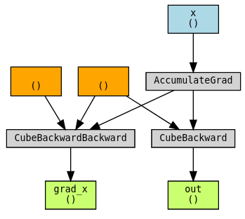
最后，双反向传播是否适用于您的自定义函数完全取决于自动求导能否跟踪反向传播过程。前两个示例展示了双反向传播可以开箱即用的情况。而在第三和第四个示例中，则演示了如何通过特定技术使反向传播过程能够被跟踪，否则是无法实现的。