注意
点击 这里 下载完整示例代码
简介 || 张量 || 自动微分 || 构建模型 || TensorBoard 支持 || 训练模型 || 模型理解
使用Pytorch进行训练
创建日期: 2021年11月30日 | 最后更新日期: 2023年5月31日 | 最后验证日期: 2024年11月5日
请跟随下方视频或在 YouTube 上观看。
介绍
在之前的视频中,我们讨论并展示了:
使用 torch.nn 模块中的神经网络层和函数构建模型
基于自动梯度计算的机制,这是梯度模型训练的核心内容。
使用TensorBoard可视化训练进度和其他活动
在本视频中,我们将为你添加一些新的工具到你的工具箱中:
我们将熟悉数据集和数据加载器的抽象概念,以及它们如何在训练循环中简化向模型提供数据的过程。
我们将讨论具体的损失函数及其适用场景。
我们将探讨PyTorch优化器,这些优化器实现了根据损失函数结果调整模型权重的算法。
最后,我们将把这些内容结合起来,看看完整的PyTorch训练循环是如何运行的。
数据集和DataLoader
The Dataset 和 DataLoader 类封装了从存储中拉取数据并在训练循环中按批次暴露数据的过程。
The Dataset 负责访问和处理单个数据实例。
The DataLoader 从 Dataset 中拉取数据实例(既可以自动拉取,也可以通过您定义的采样器进行拉取),将它们收集到批次中,并返回给您的训练循环消费。The DataLoader 可以处理所有类型的数据集,无论它们包含哪种类型的数据。
对于本教程,我们将使用TorchVision提供的Fashion-MNIST数据集。我们使用torchvision.transforms.Normalize()对图像瓷砖内容进行零中心化和标准化处理,并下载训练和验证数据分割。
import torch
import torchvision
import torchvision.transforms as transforms

# PyTorch TensorBoard support
from torch.utils.tensorboard import SummaryWriter
from datetime import datetime


transform = transforms.Compose(
    [transforms.ToTensor(),
    transforms.Normalize((0.5,), (0.5,))])

# Create datasets for training & validation, download if necessary
training_set = torchvision.datasets.FashionMNIST('./data', train=True, transform=transform, download=True)
validation_set = torchvision.datasets.FashionMNIST('./data', train=False, transform=transform, download=True)

# Create data loaders for our datasets; shuffle for training, not for validation
training_loader = torch.utils.data.DataLoader(training_set, batch_size=4, shuffle=True)
validation_loader = torch.utils.data.DataLoader(validation_set, batch_size=4, shuffle=False)

# Class labels
classes = ('T-shirt/top', 'Trouser', 'Pullover', 'Dress', 'Coat',
        'Sandal', 'Shirt', 'Sneaker', 'Bag', 'Ankle Boot')

# Report split sizes
print('Training set has {} instances'.format(len(training_set)))
print('Validation set has {} instances'.format(len(validation_set)))
Downloading http://fashion-mnist.s3-website.eu-central-1.amazonaws.com/train-images-idx3-ubyte.gz
Downloading http://fashion-mnist.s3-website.eu-central-1.amazonaws.com/train-images-idx3-ubyte.gz to ./data/FashionMNIST/raw/train-images-idx3-ubyte.gz

  0%|          | 0.00/26.4M [00:00<?, ?B/s]
  0%|          | 65.5k/26.4M [00:00<01:12, 362kB/s]
  1%|          | 197k/26.4M [00:00<00:45, 575kB/s]
  3%|3         | 852k/26.4M [00:00<00:13, 1.96MB/s]
 13%|#2        | 3.41M/26.4M [00:00<00:03, 6.75MB/s]
 32%|###1      | 8.39M/26.4M [00:00<00:01, 17.0MB/s]
 41%|####      | 10.7M/26.4M [00:00<00:00, 15.7MB/s]
 64%|######3   | 16.8M/26.4M [00:01<00:00, 22.1MB/s]
 85%|########5 | 22.5M/26.4M [00:01<00:00, 29.6MB/s]
 98%|#########8| 25.9M/26.4M [00:01<00:00, 26.2MB/s]
100%|##########| 26.4M/26.4M [00:01<00:00, 18.2MB/s]
Extracting ./data/FashionMNIST/raw/train-images-idx3-ubyte.gz to ./data/FashionMNIST/raw

Downloading http://fashion-mnist.s3-website.eu-central-1.amazonaws.com/train-labels-idx1-ubyte.gz
Downloading http://fashion-mnist.s3-website.eu-central-1.amazonaws.com/train-labels-idx1-ubyte.gz to ./data/FashionMNIST/raw/train-labels-idx1-ubyte.gz

  0%|          | 0.00/29.5k [00:00<?, ?B/s]
100%|##########| 29.5k/29.5k [00:00<00:00, 326kB/s]
Extracting ./data/FashionMNIST/raw/train-labels-idx1-ubyte.gz to ./data/FashionMNIST/raw

Downloading http://fashion-mnist.s3-website.eu-central-1.amazonaws.com/t10k-images-idx3-ubyte.gz
Downloading http://fashion-mnist.s3-website.eu-central-1.amazonaws.com/t10k-images-idx3-ubyte.gz to ./data/FashionMNIST/raw/t10k-images-idx3-ubyte.gz

  0%|          | 0.00/4.42M [00:00<?, ?B/s]
  1%|1         | 65.5k/4.42M [00:00<00:12, 360kB/s]
  4%|4         | 197k/4.42M [00:00<00:05, 731kB/s]
 11%|#1        | 492k/4.42M [00:00<00:03, 1.28MB/s]
 37%|###7      | 1.64M/4.42M [00:00<00:00, 4.18MB/s]
 87%|########6 | 3.83M/4.42M [00:00<00:00, 8.02MB/s]
100%|##########| 4.42M/4.42M [00:00<00:00, 6.06MB/s]
Extracting ./data/FashionMNIST/raw/t10k-images-idx3-ubyte.gz to ./data/FashionMNIST/raw

Downloading http://fashion-mnist.s3-website.eu-central-1.amazonaws.com/t10k-labels-idx1-ubyte.gz
Downloading http://fashion-mnist.s3-website.eu-central-1.amazonaws.com/t10k-labels-idx1-ubyte.gz to ./data/FashionMNIST/raw/t10k-labels-idx1-ubyte.gz

  0%|          | 0.00/5.15k [00:00<?, ?B/s]
100%|##########| 5.15k/5.15k [00:00<00:00, 41.4MB/s]
Extracting ./data/FashionMNIST/raw/t10k-labels-idx1-ubyte.gz to ./data/FashionMNIST/raw

Training set has 60000 instances
Validation set has 10000 instances
正如往常一样,让我们可视化数据以进行合理性检查:
import matplotlib.pyplot as plt
import numpy as np

# Helper function for inline image display
def matplotlib_imshow(img, one_channel=False):
    if one_channel:
        img = img.mean(dim=0)
    img = img / 2 + 0.5     # unnormalize
    npimg = img.numpy()
    if one_channel:
        plt.imshow(npimg, cmap="Greys")
    else:
        plt.imshow(np.transpose(npimg, (1, 2, 0)))

dataiter = iter(training_loader)
images, labels = next(dataiter)

# Create a grid from the images and show them
img_grid = torchvision.utils.make_grid(images)
matplotlib_imshow(img_grid, one_channel=True)
print('  '.join(classes[labels[j]] for j in range(4)))
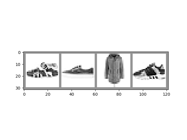
Sandal Sneaker Coat Sneaker
模型
我们在本例中使用的模型是LeNet-5的一个变种——如果你之前观看了本系列的其他视频,应该对此比较熟悉。
import torch.nn as nn
import torch.nn.functional as F

# PyTorch models inherit from torch.nn.Module
class GarmentClassifier(nn.Module):
    def __init__(self):
        super(GarmentClassifier, self).__init__()
        self.conv1 = nn.Conv2d(1, 6, 5)
        self.pool = nn.MaxPool2d(2, 2)
        self.conv2 = nn.Conv2d(6, 16, 5)
        self.fc1 = nn.Linear(16 * 4 * 4, 120)
        self.fc2 = nn.Linear(120, 84)
        self.fc3 = nn.Linear(84, 10)

    def forward(self, x):
        x = self.pool(F.relu(self.conv1(x)))
        x = self.pool(F.relu(self.conv2(x)))
        x = x.view(-1, 16 * 4 * 4)
        x = F.relu(self.fc1(x))
        x = F.relu(self.fc2(x))
        x = self.fc3(x)
        return x


model = GarmentClassifier()
损失函数
在这个例子中,我们将使用交叉熵损失。为了演示目的,我们将创建一些虚拟的输出和标签批次,将它们通过损失函数运行,并检查结果。
loss_fn = torch.nn.CrossEntropyLoss()

# NB: Loss functions expect data in batches, so we're creating batches of 4
# Represents the model's confidence in each of the 10 classes for a given input
dummy_outputs = torch.rand(4, 10)
# Represents the correct class among the 10 being tested
dummy_labels = torch.tensor([1, 5, 3, 7])

print(dummy_outputs)
print(dummy_labels)

loss = loss_fn(dummy_outputs, dummy_labels)
print('Total loss for this batch: {}'.format(loss.item()))
tensor([[0.7026, 0.1489, 0.0065, 0.6841, 0.4166, 0.3980, 0.9849, 0.6701, 0.4601,
         0.8599],
        [0.7461, 0.3920, 0.9978, 0.0354, 0.9843, 0.0312, 0.5989, 0.2888, 0.8170,
         0.4150],
        [0.8408, 0.5368, 0.0059, 0.8931, 0.3942, 0.7349, 0.5500, 0.0074, 0.0554,
         0.1537],
        [0.7282, 0.8755, 0.3649, 0.4566, 0.8796, 0.2390, 0.9865, 0.7549, 0.9105,
         0.5427]])
tensor([1, 5, 3, 7])
Total loss for this batch: 2.428950071334839
优化器
对于这个例子,我们将使用简单的随机梯度下降(SGD)带有动量。
尝试这个优化方案的一些变体也是很有益的:
学习率决定了优化器每次迭代时更新参数的步长大小。不同的学习率会对训练结果产生什么影响,特别是在准确性和收敛时间方面?
动量会在多个步骤中引导优化器朝最强梯度方向移动。改变这个值会对你的结果产生什么影响?
尝试不同的优化算法,比如平均梯度下降(SGD)、Adagrad 或 Adam。你的实验结果会有什么不同呢?
# Optimizers specified in the torch.optim package
optimizer = torch.optim.SGD(model.parameters(), lr=0.001, momentum=0.9)
训练循环
以下是执行一次训练周期的功能。它从DataLoader枚举数据,并在循环的每次迭代中执行以下操作:
从DataLoader中获取一批训练数据
清空优化器的梯度
进行推理——也就是说,为输入批次获取模型的预测
计算该组预测值与数据集中标签之间的损失
计算学习权重的反向梯度
告诉优化器执行一次学习步骤——也就是说,根据我们选择的优化算法,调整模型的学习权重,基于此批次观察到的梯度进行更新。
它每1000个批次报告一次损失。
最后,它会报告最近1000个批次的平均损失值,以便与验证运行进行比较。
def train_one_epoch(epoch_index, tb_writer):
    running_loss = 0.
    last_loss = 0.

    # Here, we use enumerate(training_loader) instead of
    # iter(training_loader) so that we can track the batch
    # index and do some intra-epoch reporting
    for i, data in enumerate(training_loader):
        # Every data instance is an input + label pair
        inputs, labels = data

        # Zero your gradients for every batch!
        optimizer.zero_grad()

        # Make predictions for this batch
        outputs = model(inputs)

        # Compute the loss and its gradients
        loss = loss_fn(outputs, labels)
        loss.backward()

        # Adjust learning weights
        optimizer.step()

        # Gather data and report
        running_loss += loss.item()
        if i % 1000 == 999:
            last_loss = running_loss / 1000 # loss per batch
            print('  batch {} loss: {}'.format(i + 1, last_loss))
            tb_x = epoch_index * len(training_loader) + i + 1
            tb_writer.add_scalar('Loss/train', last_loss, tb_x)
            running_loss = 0.

    return last_loss
每轮活动
每轮次中我们希望执行几次操作:
通过在未用于训练的数据集上检查相对损失来进行验证,并报告这一结果
保存模型的副本
在这里,我们将使用TensorBoard进行报告。这需要在命令行中启动TensorBoard,并在另一个浏览器标签页中打开它。
# Initializing in a separate cell so we can easily add more epochs to the same run
timestamp = datetime.now().strftime('%Y%m%d_%H%M%S')
writer = SummaryWriter('runs/fashion_trainer_{}'.format(timestamp))
epoch_number = 0

EPOCHS = 5

best_vloss = 1_000_000.

for epoch in range(EPOCHS):
    print('EPOCH {}:'.format(epoch_number + 1))

    # Make sure gradient tracking is on, and do a pass over the data
    model.train(True)
    avg_loss = train_one_epoch(epoch_number, writer)


    running_vloss = 0.0
    # Set the model to evaluation mode, disabling dropout and using population
    # statistics for batch normalization.
    model.eval()

    # Disable gradient computation and reduce memory consumption.
    with torch.no_grad():
        for i, vdata in enumerate(validation_loader):
            vinputs, vlabels = vdata
            voutputs = model(vinputs)
            vloss = loss_fn(voutputs, vlabels)
            running_vloss += vloss

    avg_vloss = running_vloss / (i + 1)
    print('LOSS train {} valid {}'.format(avg_loss, avg_vloss))

    # Log the running loss averaged per batch
    # for both training and validation
    writer.add_scalars('Training vs. Validation Loss',
                    { 'Training' : avg_loss, 'Validation' : avg_vloss },
                    epoch_number + 1)
    writer.flush()

    # Track best performance, and save the model's state
    if avg_vloss < best_vloss:
        best_vloss = avg_vloss
        model_path = 'model_{}_{}'.format(timestamp, epoch_number)
        torch.save(model.state_dict(), model_path)

    epoch_number += 1
EPOCH 1:
  batch 1000 loss: 1.6334228584356607
  batch 2000 loss: 0.8325267538074403
  batch 3000 loss: 0.7359380583595484
  batch 4000 loss: 0.6198329215242994
  batch 5000 loss: 0.6000315657821484
  batch 6000 loss: 0.555109024874866
  batch 7000 loss: 0.5260250487388112
  batch 8000 loss: 0.4973462742221891
  batch 9000 loss: 0.4781935699362075
  batch 10000 loss: 0.47880298678041433
  batch 11000 loss: 0.45598648857555235
  batch 12000 loss: 0.4327470133750467
  batch 13000 loss: 0.41800182418141046
  batch 14000 loss: 0.4115047634313814
  batch 15000 loss: 0.4211296908891527
LOSS train 0.4211296908891527 valid 0.414460688829422
EPOCH 2:
  batch 1000 loss: 0.3879808729066281
  batch 2000 loss: 0.35912817339546743
  batch 3000 loss: 0.38074520684120944
  batch 4000 loss: 0.3614532373107213
  batch 5000 loss: 0.36850082185724753
  batch 6000 loss: 0.3703581801643886
  batch 7000 loss: 0.38547042514081115
  batch 8000 loss: 0.37846584360170527
  batch 9000 loss: 0.3341486988377292
  batch 10000 loss: 0.3433013284947956
  batch 11000 loss: 0.35607743899174965
  batch 12000 loss: 0.3499939931873523
  batch 13000 loss: 0.33874178926000603
  batch 14000 loss: 0.35130289171106416
  batch 15000 loss: 0.3394507191307202
LOSS train 0.3394507191307202 valid 0.3581162691116333
EPOCH 3:
  batch 1000 loss: 0.3319729989422485
  batch 2000 loss: 0.29558994361863006
  batch 3000 loss: 0.3107374766407593
  batch 4000 loss: 0.3298987646112146
  batch 5000 loss: 0.30858693152241906
  batch 6000 loss: 0.33916381367447684
  batch 7000 loss: 0.3105102765217889
  batch 8000 loss: 0.3011080777524912
  batch 9000 loss: 0.3142058177240979
  batch 10000 loss: 0.31458891937109
  batch 11000 loss: 0.31527258940579483
  batch 12000 loss: 0.31501667268342864
  batch 13000 loss: 0.3011875962628328
  batch 14000 loss: 0.30012811454350596
  batch 15000 loss: 0.31833117976446373
LOSS train 0.31833117976446373 valid 0.3307691514492035
EPOCH 4:
  batch 1000 loss: 0.2786161053752294
  batch 2000 loss: 0.27965198021690596
  batch 3000 loss: 0.28595415444140965
  batch 4000 loss: 0.292985666413857
  batch 5000 loss: 0.3069892351147719
  batch 6000 loss: 0.29902250939945224
  batch 7000 loss: 0.2863366014406201
  batch 8000 loss: 0.2655441066541243
  batch 9000 loss: 0.3045048695363293
  batch 10000 loss: 0.27626545656517554
  batch 11000 loss: 0.2808379335970967
  batch 12000 loss: 0.29241049340573955
  batch 13000 loss: 0.28030834131941446
  batch 14000 loss: 0.2983542350126445
  batch 15000 loss: 0.3009556676162611
LOSS train 0.3009556676162611 valid 0.41686952114105225
EPOCH 5:
  batch 1000 loss: 0.2614263167564495
  batch 2000 loss: 0.2587047562422049
  batch 3000 loss: 0.2642477260621345
  batch 4000 loss: 0.2825975873669813
  batch 5000 loss: 0.26987933717705165
  batch 6000 loss: 0.2759250026817317
  batch 7000 loss: 0.26055969463163275
  batch 8000 loss: 0.29164007206353565
  batch 9000 loss: 0.2893096504513578
  batch 10000 loss: 0.2486029507305684
  batch 11000 loss: 0.2732803234480907
  batch 12000 loss: 0.27927226484491985
  batch 13000 loss: 0.2686819267635074
  batch 14000 loss: 0.24746483912148323
  batch 15000 loss: 0.27903492261294194
LOSS train 0.27903492261294194 valid 0.31206756830215454
要加载保存的模型版本:
saved_model = GarmentClassifier()
saved_model.load_state_dict(torch.load(PATH))
一旦您加载了模型,它就可以用于您需要的所有方面——更多的训练、推理或分析。
请注意,如果您模型的构造参数会影响模型结构,在保存模型的状态时,您需要提供这些参数并在加载模型时将其配置得与保存时一致。
其他资源
在 pytorch.org 上查看有关 数据工具 的文档,包括 Dataset 和 DataLoader
关于在GPU训练中使用固定内存的说明
Documentation on the datasets available in TorchVision, TorchText, and TorchAudio
PyTorch 中可用的 损失函数 的文档
关于 torch.optim 包的文档,其中包括优化器及相关工具,例如学习率调度
一个关于保存和加载模型的详细教程
Pytorch.org网站的教程部分包含各种训练任务的教程,包括不同领域的分类、生成对抗网络、强化学习等更多内容
脚本总运行时间: (5分钟 0.727秒)