注意
点击 这里 下载完整示例代码
音频特征提取
作者: Moto Hira
torchaudio 实现了音频领域常用的特征提取方法。它们在 torchaudio.functional 和
torchaudio.transforms 中可用。
functional 以独立函数的形式实现功能。
它们是无状态的。
transforms 将功能实现为对象,
使用来自 functional 和 torch.nn.Module 的实现。
它们可以使用 TorchScript 进行序列化。
import torch
import torchaudio
import torchaudio.functional as F
import torchaudio.transforms as T

print(torch.__version__)
print(torchaudio.__version__)
2.0.0
2.0.1
准备
注意
在 Google Colab 中运行本教程时,请安装所需的软件包
!pip install librosa
from IPython.display import Audio
import librosa
import matplotlib.pyplot as plt
from torchaudio.utils import download_asset

torch.random.manual_seed(0)

SAMPLE_SPEECH = download_asset("tutorial-assets/Lab41-SRI-VOiCES-src-sp0307-ch127535-sg0042.wav")


def plot_waveform(waveform, sr, title="Waveform"):
    waveform = waveform.numpy()

    num_channels, num_frames = waveform.shape
    time_axis = torch.arange(0, num_frames) / sr

    figure, axes = plt.subplots(num_channels, 1)
    axes.plot(time_axis, waveform[0], linewidth=1)
    axes.grid(True)
    figure.suptitle(title)
    plt.show(block=False)


def plot_spectrogram(specgram, title=None, ylabel="freq_bin"):
    fig, axs = plt.subplots(1, 1)
    axs.set_title(title or "Spectrogram (db)")
    axs.set_ylabel(ylabel)
    axs.set_xlabel("frame")
    im = axs.imshow(librosa.power_to_db(specgram), origin="lower", aspect="auto")
    fig.colorbar(im, ax=axs)
    plt.show(block=False)


def plot_fbank(fbank, title=None):
    fig, axs = plt.subplots(1, 1)
    axs.set_title(title or "Filter bank")
    axs.imshow(fbank, aspect="auto")
    axs.set_ylabel("frequency bin")
    axs.set_xlabel("mel bin")
    plt.show(block=False)
音频功能概述
下图展示了常见音频特征与用于生成它们的 torchaudio API 之间的关系。
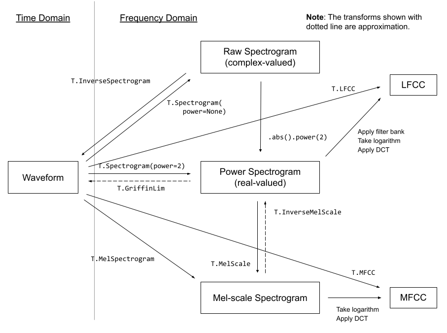
如需查看完整的可用功能列表,请参阅文档。
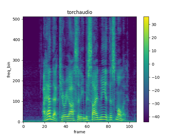
频谱图
要获取音频信号随时间变化的频率组成,
你可以使用 torchaudio.transforms.Spectrogram()。
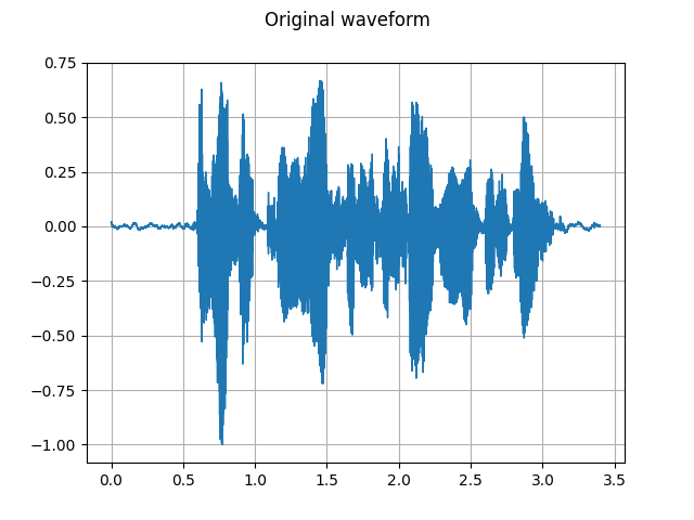
SPEECH_WAVEFORM, SAMPLE_RATE = torchaudio.load(SAMPLE_SPEECH)

plot_waveform(SPEECH_WAVEFORM, SAMPLE_RATE, title="Original waveform")
Audio(SPEECH_WAVEFORM.numpy(), rate=SAMPLE_RATE)
n_fft = 1024
win_length = None
hop_length = 512

# Define transform
spectrogram = T.Spectrogram(
    n_fft=n_fft,
    win_length=win_length,
    hop_length=hop_length,
    center=True,
    pad_mode="reflect",
    power=2.0,
)
# Perform transform
spec = spectrogram(SPEECH_WAVEFORM)
plot_spectrogram(spec[0], title="torchaudio")
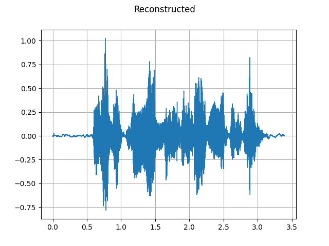
GriffinLim
要从频谱图恢复波形,您可以使用 GriffinLim。
torch.random.manual_seed(0)

n_fft = 1024
win_length = None
hop_length = 512

spec = T.Spectrogram(
    n_fft=n_fft,
    win_length=win_length,
    hop_length=hop_length,
)(SPEECH_WAVEFORM)
griffin_lim = T.GriffinLim(
    n_fft=n_fft,
    win_length=win_length,
    hop_length=hop_length,
)
reconstructed_waveform = griffin_lim(spec)
plot_waveform(reconstructed_waveform, SAMPLE_RATE, title="Reconstructed")
Audio(reconstructed_waveform, rate=SAMPLE_RATE)
梅尔滤波器组
torchaudio.functional.melscale_fbanks() 生成用于将频率分 bin 转换为梅尔刻度分 bin 的滤波器组。
由于此函数不需要输入音频/特征,因此在 torchaudio.transforms() 中没有等效的转换。
n_fft = 256
n_mels = 64
sample_rate = 6000

mel_filters = F.melscale_fbanks(
    int(n_fft // 2 + 1),
    n_mels=n_mels,
    f_min=0.0,
    f_max=sample_rate / 2.0,
    sample_rate=sample_rate,
    norm="slaney",
)
plot_fbank(mel_filters, "Mel Filter Bank - torchaudio")

与librosa的对比
作为参考,以下是使用 librosa 获取 mel 滤波器组的等效方法。
mel_filters_librosa = librosa.filters.mel(
    sr=sample_rate,
    n_fft=n_fft,
    n_mels=n_mels,
    fmin=0.0,
    fmax=sample_rate / 2.0,
    norm="slaney",
    htk=True,
).T
plot_fbank(mel_filters_librosa, "Mel Filter Bank - librosa")

mse = torch.square(mel_filters - mel_filters_librosa).mean().item()
print("Mean Square Difference: ", mse)
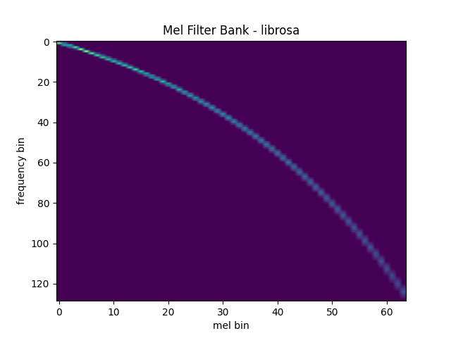
Mean Square Difference: 3.934872696751886e-17
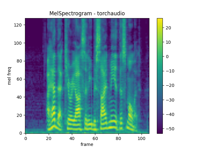
MelSpectrogram
生成一个梅尔频谱图涉及生成一个频谱图
并进行梅尔尺度转换。在 torchaudio,
torchaudio.transforms.MelSpectrogram() 提供了
此功能。
n_fft = 1024
win_length = None
hop_length = 512
n_mels = 128

mel_spectrogram = T.MelSpectrogram(
    sample_rate=sample_rate,
    n_fft=n_fft,
    win_length=win_length,
    hop_length=hop_length,
    center=True,
    pad_mode="reflect",
    power=2.0,
    norm="slaney",
    onesided=True,
    n_mels=n_mels,
    mel_scale="htk",
)

melspec = mel_spectrogram(SPEECH_WAVEFORM)
/usr/local/envs/python3.8/lib/python3.8/site-packages/torchaudio/transforms/_transforms.py:611: UserWarning: Argument 'onesided' has been deprecated and has no influence on the behavior of this module.
  warnings.warn(
plot_spectrogram(melspec[0], title="MelSpectrogram - torchaudio", ylabel="mel freq")
与librosa的对比
作为参考,以下是使用 librosa 生成梅尔尺度频谱图的等效方法。
melspec_librosa = librosa.feature.melspectrogram(
    y=SPEECH_WAVEFORM.numpy()[0],
    sr=sample_rate,
    n_fft=n_fft,
    hop_length=hop_length,
    win_length=win_length,
    center=True,
    pad_mode="reflect",
    power=2.0,
    n_mels=n_mels,
    norm="slaney",
    htk=True,
)
plot_spectrogram(melspec_librosa, title="MelSpectrogram - librosa", ylabel="mel freq")

mse = torch.square(melspec - melspec_librosa).mean().item()
print("Mean Square Difference: ", mse)

Mean Square Difference: 1.2913579094941952e-09
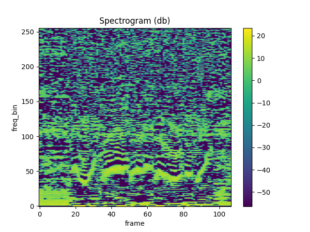
MFCC
n_fft = 2048
win_length = None
hop_length = 512
n_mels = 256
n_mfcc = 256

mfcc_transform = T.MFCC(
    sample_rate=sample_rate,
    n_mfcc=n_mfcc,
    melkwargs={
        "n_fft": n_fft,
        "n_mels": n_mels,
        "hop_length": hop_length,
        "mel_scale": "htk",
    },
)

mfcc = mfcc_transform(SPEECH_WAVEFORM)
plot_spectrogram(mfcc[0])
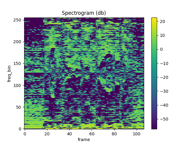
与librosa的对比
melspec = librosa.feature.melspectrogram(
    y=SPEECH_WAVEFORM.numpy()[0],
    sr=sample_rate,
    n_fft=n_fft,
    win_length=win_length,
    hop_length=hop_length,
    n_mels=n_mels,
    htk=True,
    norm=None,
)

mfcc_librosa = librosa.feature.mfcc(
    S=librosa.core.spectrum.power_to_db(melspec),
    n_mfcc=n_mfcc,
    dct_type=2,
    norm="ortho",
)
plot_spectrogram(mfcc_librosa)

mse = torch.square(mfcc - mfcc_librosa).mean().item()
print("Mean Square Difference: ", mse)

Mean Square Difference: 0.8103961944580078
LFCC
n_fft = 2048
win_length = None
hop_length = 512
n_lfcc = 256

lfcc_transform = T.LFCC(
    sample_rate=sample_rate,
    n_lfcc=n_lfcc,
    speckwargs={
        "n_fft": n_fft,
        "win_length": win_length,
        "hop_length": hop_length,
    },
)

lfcc = lfcc_transform(SPEECH_WAVEFORM)
plot_spectrogram(lfcc[0])
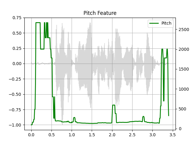
简介
pitch = F.detect_pitch_frequency(SPEECH_WAVEFORM, SAMPLE_RATE)
def plot_pitch(waveform, sr, pitch):
    figure, axis = plt.subplots(1, 1)
    axis.set_title("Pitch Feature")
    axis.grid(True)

    end_time = waveform.shape[1] / sr
    time_axis = torch.linspace(0, end_time, waveform.shape[1])
    axis.plot(time_axis, waveform[0], linewidth=1, color="gray", alpha=0.3)

    axis2 = axis.twinx()
    time_axis = torch.linspace(0, end_time, pitch.shape[1])
    axis2.plot(time_axis, pitch[0], linewidth=2, label="Pitch", color="green")

    axis2.legend(loc=0)
    plt.show(block=False)


plot_pitch(SPEECH_WAVEFORM, SAMPLE_RATE, pitch)
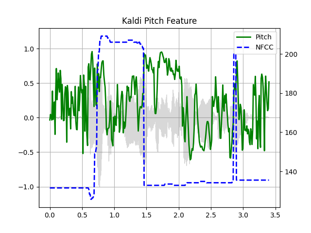
Kaldi 音高(测试版)
Kaldi 音高特征 [1] 是一种针对自动语音识别 (ASR) 应用进行优化的音高检测机制。这是 torchaudio 中的测试版功能,并作为 torchaudio.functional.compute_kaldi_pitch() 提供。
一种针对自动语音识别优化的音高提取算法
Ghahremani, B. BabaAli, D. Povey, K. Riedhammer, J. Trmal 和 S. Khudanpur
2014 IEEE国际声学、语音和信号处理会议 (ICASSP), 佛罗伦萨, 2014, pp. 2494-2498, doi: 10.1109/ICASSP.2014.6854049. [摘要], [论文]
pitch_feature = F.compute_kaldi_pitch(SPEECH_WAVEFORM, SAMPLE_RATE)
pitch, nfcc = pitch_feature[..., 0], pitch_feature[..., 1]
def plot_kaldi_pitch(waveform, sr, pitch, nfcc):
    _, axis = plt.subplots(1, 1)
    axis.set_title("Kaldi Pitch Feature")
    axis.grid(True)

    end_time = waveform.shape[1] / sr
    time_axis = torch.linspace(0, end_time, waveform.shape[1])
    axis.plot(time_axis, waveform[0], linewidth=1, color="gray", alpha=0.3)

    time_axis = torch.linspace(0, end_time, pitch.shape[1])
    ln1 = axis.plot(time_axis, pitch[0], linewidth=2, label="Pitch", color="green")
    axis.set_ylim((-1.3, 1.3))

    axis2 = axis.twinx()
    time_axis = torch.linspace(0, end_time, nfcc.shape[1])
    ln2 = axis2.plot(time_axis, nfcc[0], linewidth=2, label="NFCC", color="blue", linestyle="--")

    lns = ln1 + ln2
    labels = [l.get_label() for l in lns]
    axis.legend(lns, labels, loc=0)
    plt.show(block=False)


plot_kaldi_pitch(SPEECH_WAVEFORM, SAMPLE_RATE, pitch, nfcc)
脚本的总运行时间: ( 0 分钟 11.902 秒)