注意

点击这里下载完整示例代码

使用CTC解码器进行ASR推理¶

作者: Caroline Chen

本教程演示了如何使用带有词典约束和 KenLM 语言模型支持的 CTC 贝叶斯搜索解码器进行语音识别推理。我们将在一个使用 CTC 损失训练的预训练 wav2vec 2.0 模型上展示这一过程。

概述¶

束搜索解码通过迭代扩展文本假设（束），使用下一个可能的字符，并在每个时间步仅保留得分最高的假设。可以将语言模型纳入评分计算中，添加词典约束可以限制假设的下一个可能标记，使得只能生成词典中的词语。

底层实现是从 Flashlight 的束搜索解码器移植而来的。解码器优化的数学公式可以在 Wav2Letter 论文中找到，更详细的算法可以在这篇博客中找到。

使用带有语言模型和词典约束的CTC Beam Search解码器运行ASR推理需要以下组件

声学模型：从音频波形预测语音特征的模型
Tokens: 语音模型可能预测的标记
词典：可能的单词与对应标记序列之间的映射
语言模型 (LM): 使用 KenLM 库训练的 n-gram 语言模型，或继承自 CTCDecoderLM 的自定义语言模型

声学模型与设置¶

首先我们导入必要的工具并获取我们正在使用的数据

import torch
import torchaudio

print(torch.__version__)
print(torchaudio.__version__)

2.0.0
2.0.1

import time
from typing import List

import IPython
import matplotlib.pyplot as plt
from torchaudio.models.decoder import ctc_decoder
from torchaudio.utils import download_asset

我们使用在 Wav2Vec 2.0 基础模型上微调的10分钟 LibriSpeech 数据集，可以通过 torchaudio.pipelines.WAV2VEC2_ASR_BASE_10M 加载。有关在 torchaudio 中运行 Wav2Vec 2.0 语音识别流水线的更多详细信息，请参阅本教程。

bundle = torchaudio.pipelines.WAV2VEC2_ASR_BASE_10M
acoustic_model = bundle.get_model()

Downloading: "https://download.pytorch.org/torchaudio/models/wav2vec2_fairseq_base_ls960_asr_ll10m.pth" to /root/.cache/torch/hub/checkpoints/wav2vec2_fairseq_base_ls960_asr_ll10m.pth

  0%|          | 0.00/360M [00:00<?, ?B/s]
 11%|#1        | 41.3M/360M [00:00<00:00, 433MB/s]
 23%|##2       | 82.6M/360M [00:00<00:00, 398MB/s]
 35%|###4      | 125M/360M [00:00<00:00, 420MB/s]
 47%|####7     | 169M/360M [00:00<00:00, 436MB/s]
 59%|#####8    | 212M/360M [00:00<00:00, 441MB/s]
 71%|#######   | 255M/360M [00:00<00:00, 441MB/s]
 83%|########2 | 298M/360M [00:00<00:00, 447MB/s]
 95%|#########4| 341M/360M [00:00<00:00, 448MB/s]
100%|##########| 360M/360M [00:00<00:00, 400MB/s]

我们将从 LibriSpeech test-other 数据集中加载一个样本。

speech_file = download_asset("tutorial-assets/ctc-decoding/1688-142285-0007.wav")

IPython.display.Audio(speech_file)

  0%|          | 0.00/441k [00:00<?, ?B/s]
100%|##########| 441k/441k [00:00<00:00, 124MB/s]

该音频文件对应的文本是

i really was very much afraid of showing him how much shocked i was at some parts of what he said

waveform, sample_rate = torchaudio.load(speech_file)

if sample_rate != bundle.sample_rate:
    waveform = torchaudio.functional.resample(waveform, sample_rate, bundle.sample_rate)

文件和数据用于解码器¶

接下来，我们加载词元、词典和语言模型数据，这些数据用于解码器根据声学模型的输出预测词语。LibriSpeech 数据集的预训练文件可以通过 torchaudio 下载，或者用户也可以提供自己的文件。

Tokens¶

这些符号是声学模型可以预测的可能符号，包括空白符号和静音符号。它们既可以作为文件传入，每行对应相同索引的符号，也可以作为符号列表传入，每个符号映射到唯一的索引。

# tokens.txt
_
|
e
t
...

tokens = [label.lower() for label in bundle.get_labels()]
print(tokens)

['-', '|', 'e', 't', 'a', 'o', 'n', 'i', 'h', 's', 'r', 'd', 'l', 'u', 'm', 'w', 'c', 'f', 'g', 'y', 'p', 'b', 'v', 'k', "'", 'x', 'j', 'q', 'z']

术语表¶

词典是将单词映射到其对应标记序列的映射，用于将解码器的搜索空间限制为仅来自词典中的单词。词典文件的预期格式是每行一个单词，单词后跟由空格分隔的标记。

# lexcion.txt
a a |
able a b l e |
about a b o u t |
...
...

语言模型¶

在解码过程中，可以使用语言模型来改进结果，方法是将代表序列可能性的语言模型得分纳入到束搜索计算中。下面，我们将概述支持用于解码的不同形式的语言模型。

无语言模型¶

要创建一个不带语言模型的解码器实例，请在初始化解码器时将 lm=None 设置为参数。

KenLM¶

这是一个使用 KenLM库训练的n-gram语言模型。可以使用 .arpa 或者二进制化的 .bin 语言模型，但推荐使用二进制格式以加快加载速度。

本教程中使用的语言模型是一个使用 LibriSpeech训练的4-gram KenLM。

自定义语言模型¶

用户可以使用 Python 定义自己的自定义语言模型，无论是统计语言模型还是神经网络语言模型，只需使用 CTCDecoderLM 和 CTCDecoderLMState。

例如，以下代码创建了一个围绕 PyTorch torch.nn.Module 语言模型的基本包装器。

from torchaudio.models.decoder import CTCDecoderLM, CTCDecoderLMState


class CustomLM(CTCDecoderLM):
    """Create a Python wrapper around `language_model` to feed to the decoder."""
    def __init__(self, language_model: torch.nn.Module):
        CTCDecoderLM.__init__(self)
        self.language_model = language_model
        self.sil = -1  # index for silent token in the language model
        self.states = {}

        language_model.eval()

    def start(self, start_with_nothing: bool = False):
        state = CTCDecoderLMState()
        with torch.no_grad():
            score = self.language_model(self.sil)

        self.states[state] = score
        return state

    def score(self, state: CTCDecoderLMState, token_index: int):
        outstate = state.child(token_index)
        if outstate not in self.states:
            score = self.language_model(token_index)
            self.states[outstate] = score
        score = self.states[outstate]

        return outstate, score

    def finish(self, state: CTCDecoderLMState):
        return self.score(state, self.sil)

下载预训练文件¶

LibriSpeech 数据集的预训练文件可以使用 download_pretrained_files()下载。

注意：由于语言模型可能较大，此单元格运行可能需要几分钟。

from torchaudio.models.decoder import download_pretrained_files

files = download_pretrained_files("librispeech-4-gram")

print(files)

  0%|          | 0.00/4.97M [00:00<?, ?B/s]
100%|##########| 4.97M/4.97M [00:00<00:00, 376MB/s]

  0%|          | 0.00/57.0 [00:00<?, ?B/s]
100%|##########| 57.0/57.0 [00:00<00:00, 57.7kB/s]

  0%|          | 0.00/2.91G [00:00<?, ?B/s]
  1%|1         | 37.9M/2.91G [00:00<00:07, 398MB/s]
  3%|2         | 75.9M/2.91G [00:00<00:08, 380MB/s]
  4%|4         | 119M/2.91G [00:00<00:07, 414MB/s]
  5%|5         | 163M/2.91G [00:00<00:06, 431MB/s]
  7%|6         | 206M/2.91G [00:00<00:06, 436MB/s]
  8%|8         | 249M/2.91G [00:00<00:06, 443MB/s]
 10%|9         | 291M/2.91G [00:00<00:06, 419MB/s]
 11%|#1        | 334M/2.91G [00:00<00:06, 428MB/s]
 13%|#2        | 376M/2.91G [00:00<00:06, 432MB/s]
 14%|#4        | 417M/2.91G [00:01<00:06, 418MB/s]
 15%|#5        | 461M/2.91G [00:01<00:06, 430MB/s]
 17%|#6        | 502M/2.91G [00:01<00:06, 396MB/s]
 18%|#8        | 541M/2.91G [00:01<00:06, 395MB/s]
 19%|#9        | 581M/2.91G [00:01<00:06, 403MB/s]
 21%|##        | 621M/2.91G [00:01<00:06, 409MB/s]
 22%|##2       | 661M/2.91G [00:01<00:05, 410MB/s]
 23%|##3       | 700M/2.91G [00:01<00:05, 403MB/s]
 25%|##4       | 740M/2.91G [00:01<00:05, 408MB/s]
 26%|##6       | 779M/2.91G [00:01<00:05, 408MB/s]
 27%|##7       | 818M/2.91G [00:02<00:05, 408MB/s]
 29%|##8       | 861M/2.91G [00:02<00:05, 418MB/s]
 30%|###       | 903M/2.91G [00:02<00:05, 427MB/s]
 32%|###1      | 946M/2.91G [00:02<00:04, 435MB/s]
 33%|###3      | 988M/2.91G [00:02<00:04, 434MB/s]
 35%|###4      | 1.01G/2.91G [00:02<00:04, 431MB/s]
 36%|###5      | 1.05G/2.91G [00:02<00:04, 422MB/s]
 37%|###7      | 1.09G/2.91G [00:02<00:04, 429MB/s]
 39%|###8      | 1.13G/2.91G [00:02<00:04, 434MB/s]
 40%|####      | 1.17G/2.91G [00:02<00:04, 433MB/s]
 42%|####1     | 1.21G/2.91G [00:03<00:04, 432MB/s]
 43%|####2     | 1.25G/2.91G [00:03<00:04, 430MB/s]
 44%|####4     | 1.29G/2.91G [00:03<00:04, 412MB/s]
 46%|####5     | 1.33G/2.91G [00:03<00:04, 422MB/s]
 47%|####7     | 1.37G/2.91G [00:03<00:03, 431MB/s]
 49%|####8     | 1.42G/2.91G [00:03<00:03, 437MB/s]
 50%|#####     | 1.46G/2.91G [00:03<00:03, 439MB/s]
 51%|#####1    | 1.50G/2.91G [00:03<00:03, 442MB/s]
 53%|#####2    | 1.54G/2.91G [00:03<00:03, 442MB/s]
 54%|#####4    | 1.58G/2.91G [00:04<00:03, 443MB/s]
 56%|#####5    | 1.62G/2.91G [00:04<00:03, 445MB/s]
 57%|#####7    | 1.66G/2.91G [00:04<00:03, 441MB/s]
 59%|#####8    | 1.71G/2.91G [00:04<00:02, 442MB/s]
 60%|######    | 1.75G/2.91G [00:04<00:02, 442MB/s]
 61%|######1   | 1.79G/2.91G [00:04<00:02, 443MB/s]
 63%|######2   | 1.83G/2.91G [00:04<00:02, 442MB/s]
 64%|######4   | 1.87G/2.91G [00:04<00:02, 444MB/s]
 66%|######5   | 1.91G/2.91G [00:04<00:02, 446MB/s]
 67%|######7   | 1.96G/2.91G [00:04<00:02, 449MB/s]
 69%|######8   | 2.00G/2.91G [00:05<00:02, 450MB/s]
 70%|#######   | 2.04G/2.91G [00:05<00:02, 450MB/s]
 72%|#######1  | 2.08G/2.91G [00:05<00:01, 450MB/s]
 73%|#######2  | 2.12G/2.91G [00:05<00:01, 450MB/s]
 74%|#######4  | 2.17G/2.91G [00:05<00:01, 450MB/s]
 76%|#######5  | 2.21G/2.91G [00:05<00:01, 440MB/s]
 77%|#######7  | 2.25G/2.91G [00:05<00:01, 438MB/s]
 79%|#######8  | 2.29G/2.91G [00:05<00:01, 441MB/s]
 80%|########  | 2.33G/2.91G [00:05<00:01, 443MB/s]
 82%|########1 | 2.37G/2.91G [00:05<00:01, 445MB/s]
 83%|########3 | 2.42G/2.91G [00:06<00:01, 445MB/s]
 84%|########4 | 2.46G/2.91G [00:06<00:01, 447MB/s]
 86%|########5 | 2.50G/2.91G [00:06<00:01, 400MB/s]
 87%|########7 | 2.54G/2.91G [00:06<00:00, 408MB/s]
 89%|########8 | 2.58G/2.91G [00:06<00:00, 420MB/s]
 90%|######### | 2.62G/2.91G [00:06<00:00, 428MB/s]
 92%|#########1| 2.66G/2.91G [00:06<00:00, 434MB/s]
 93%|#########3| 2.71G/2.91G [00:06<00:00, 439MB/s]
 94%|#########4| 2.75G/2.91G [00:06<00:00, 436MB/s]
 96%|#########5| 2.79G/2.91G [00:06<00:00, 441MB/s]
 97%|#########7| 2.83G/2.91G [00:07<00:00, 444MB/s]
 99%|#########8| 2.87G/2.91G [00:07<00:00, 444MB/s]
100%|##########| 2.91G/2.91G [00:07<00:00, 431MB/s]
PretrainedFiles(lexicon='/root/.cache/torch/hub/torchaudio/decoder-assets/librispeech-4-gram/lexicon.txt', tokens='/root/.cache/torch/hub/torchaudio/decoder-assets/librispeech-4-gram/tokens.txt', lm='/root/.cache/torch/hub/torchaudio/decoder-assets/librispeech-4-gram/lm.bin')

构建解码器¶

在本教程中，我们构建了一个束搜索解码器和一个贪婪解码器以进行比较。

束搜索解码器¶

解码器可以使用工厂函数 ctc_decoder()构建。除了前面提到的组件外，它还接受各种束搜索解码参数和令牌/单词参数。

通过向 None 参数传入 lm，此解码器也可以在不使用语言模型的情况下运行。

LM_WEIGHT = 3.23
WORD_SCORE = -0.26

beam_search_decoder = ctc_decoder(
    lexicon=files.lexicon,
    tokens=files.tokens,
    lm=files.lm,
    nbest=3,
    beam_size=1500,
    lm_weight=LM_WEIGHT,
    word_score=WORD_SCORE,
)

贪婪解码器¶

class GreedyCTCDecoder(torch.nn.Module):
    def __init__(self, labels, blank=0):
        super().__init__()
        self.labels = labels
        self.blank = blank

    def forward(self, emission: torch.Tensor) -> List[str]:
        """Given a sequence emission over labels, get the best path
        Args:
          emission (Tensor): Logit tensors. Shape `[num_seq, num_label]`.

        Returns:
          List[str]: The resulting transcript
        """
        indices = torch.argmax(emission, dim=-1)  # [num_seq,]
        indices = torch.unique_consecutive(indices, dim=-1)
        indices = [i for i in indices if i != self.blank]
        joined = "".join([self.labels[i] for i in indices])
        return joined.replace("|", " ").strip().split()


greedy_decoder = GreedyCTCDecoder(tokens)

运行推理¶

现在我们已经拥有了数据、声学模型和解码器，可以执行推理。束搜索解码器的输出类型为 CTCHypothesis，包含预测的 token ID、对应的单词（如果提供了词典）、假设分数以及与 token ID 对应的时间步。回顾一下，与波形对应的转录文本是

i really was very much afraid of showing him how much shocked i was at some parts of what he said

actual_transcript = "i really was very much afraid of showing him how much shocked i was at some parts of what he said"
actual_transcript = actual_transcript.split()

emission, _ = acoustic_model(waveform)

贪婪解码器给出以下结果。

greedy_result = greedy_decoder(emission[0])
greedy_transcript = " ".join(greedy_result)
greedy_wer = torchaudio.functional.edit_distance(actual_transcript, greedy_result) / len(actual_transcript)

print(f"Transcript: {greedy_transcript}")
print(f"WER: {greedy_wer}")

Transcript: i reily was very much affrayd of showing him howmuch shoktd i wause at some parte of what he seid
WER: 0.38095238095238093

使用束搜索解码器：

beam_search_result = beam_search_decoder(emission)
beam_search_transcript = " ".join(beam_search_result[0][0].words).strip()
beam_search_wer = torchaudio.functional.edit_distance(actual_transcript, beam_search_result[0][0].words) / len(
    actual_transcript
)

print(f"Transcript: {beam_search_transcript}")
print(f"WER: {beam_search_wer}")

Transcript: i really was very much afraid of showing him how much shocked i was at some part of what he said
WER: 0.047619047619047616

注意

如果未向解码器提供词典，输出假设的 words 字段将为空。要检索无词典解码的转录文本，您可以执行以下操作以获取令牌索引，将它们转换为原始令牌，然后将它们连接在一起。

tokens_str = "".join(beam_search_decoder.idxs_to_tokens(beam_search_result[0][0].tokens))
transcript = " ".join(tokens_str.split("|"))

我们发现，使用词典约束束搜索解码器生成的转录结果更为准确，由真实单词组成；而贪婪解码器则可能预测出拼写错误的单词，如"affrayd"和"shoktd"。

时间步对齐¶

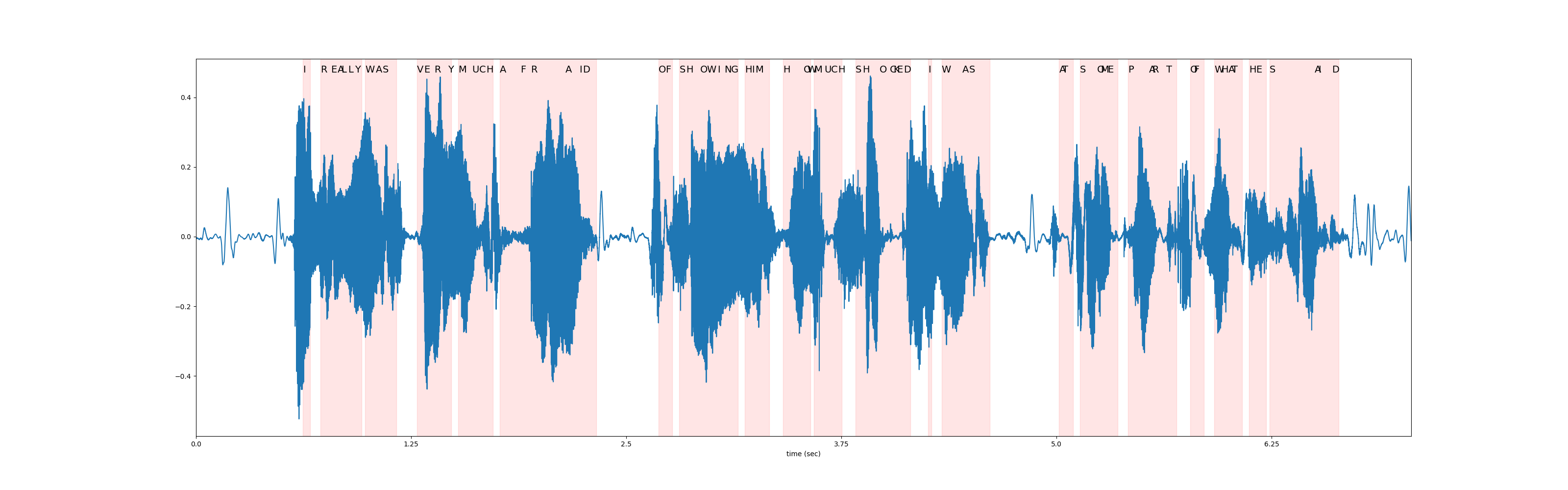
请注意，生成的假设的组成部分之一是与时令 ID 对应的时间步。

timesteps = beam_search_result[0][0].timesteps
predicted_tokens = beam_search_decoder.idxs_to_tokens(beam_search_result[0][0].tokens)

print(predicted_tokens, len(predicted_tokens))
print(timesteps, timesteps.shape[0])

['|', 'i', '|', 'r', 'e', 'a', 'l', 'l', 'y', '|', 'w', 'a', 's', '|', 'v', 'e', 'r', 'y', '|', 'm', 'u', 'c', 'h', '|', 'a', 'f', 'r', 'a', 'i', 'd', '|', 'o', 'f', '|', 's', 'h', 'o', 'w', 'i', 'n', 'g', '|', 'h', 'i', 'm', '|', 'h', 'o', 'w', '|', 'm', 'u', 'c', 'h', '|', 's', 'h', 'o', 'c', 'k', 'e', 'd', '|', 'i', '|', 'w', 'a', 's', '|', 'a', 't', '|', 's', 'o', 'm', 'e', '|', 'p', 'a', 'r', 't', '|', 'o', 'f', '|', 'w', 'h', 'a', 't', '|', 'h', 'e', '|', 's', 'a', 'i', 'd', '|', '|'] 99
tensor([  0,  31,  33,  36,  39,  41,  42,  44,  46,  48,  49,  52,  54,  58,
         64,  66,  69,  73,  74,  76,  80,  82,  84,  86,  88,  94,  97, 107,
        111, 112, 116, 134, 136, 138, 140, 142, 146, 148, 151, 153, 155, 157,
        159, 161, 162, 166, 170, 176, 177, 178, 179, 182, 184, 186, 187, 191,
        193, 198, 201, 202, 203, 205, 207, 212, 213, 216, 222, 224, 230, 250,
        251, 254, 256, 261, 262, 264, 267, 270, 276, 277, 281, 284, 288, 289,
        292, 295, 297, 299, 300, 303, 305, 307, 310, 311, 324, 325, 329, 331,
        353], dtype=torch.int32) 99

在下图中，我们可视化了相对于原始波形的 token 时间步对齐情况。

def plot_alignments(waveform, emission, tokens, timesteps):
    fig, ax = plt.subplots(figsize=(32, 10))

    ax.plot(waveform)

    ratio = waveform.shape[0] / emission.shape[1]
    word_start = 0

    for i in range(len(tokens)):
        if i != 0 and tokens[i - 1] == "|":
            word_start = timesteps[i]
        if tokens[i] != "|":
            plt.annotate(tokens[i].upper(), (timesteps[i] * ratio, waveform.max() * 1.02), size=14)
        elif i != 0:
            word_end = timesteps[i]
            ax.axvspan(word_start * ratio, word_end * ratio, alpha=0.1, color="red")

    xticks = ax.get_xticks()
    plt.xticks(xticks, xticks / bundle.sample_rate)
    ax.set_xlabel("time (sec)")
    ax.set_xlim(0, waveform.shape[0])


plot_alignments(waveform[0], emission, predicted_tokens, timesteps)

Beam Search Decoder Parameters¶

在本节中，我们将更深入地探讨一些不同的参数和权衡。有关可自定义参数的完整列表，请参阅 documentation。

辅助函数¶

def print_decoded(decoder, emission, param, param_value):
    start_time = time.monotonic()
    result = decoder(emission)
    decode_time = time.monotonic() - start_time

    transcript = " ".join(result[0][0].words).lower().strip()
    score = result[0][0].score
    print(f"{param} {param_value:<3}: {transcript} (score: {score:.2f}; {decode_time:.4f} secs)")

nbest¶

此参数指示要返回的最佳假设数量，这是贪婪解码器无法实现的属性。例如，通过在之前构建束搜索解码器时将 nbest=3 设置为该值，我们现在可以访问得分最高的前 3 个假设。

for i in range(3):
    transcript = " ".join(beam_search_result[0][i].words).strip()
    score = beam_search_result[0][i].score
    print(f"{transcript} (score: {score})")

i really was very much afraid of showing him how much shocked i was at some part of what he said (score: 3699.8241478490795)
i really was very much afraid of showing him how much shocked i was at some parts of what he said (score: 3697.8584095108477)
i reply was very much afraid of showing him how much shocked i was at some part of what he said (score: 3695.01579982042)

束宽¶

beam_size 参数决定了在每个解码步骤后保留的最佳假设的最大数量。使用更大的束宽（beam size）可以探索更大范围的潜在假设，从而可能生成得分更高的假设，但这在计算上更为昂贵，并且在达到某个临界点后不会带来额外的收益。

在下方的示例中，我们看到随着束宽从 1 增加到 5 再到 50，解码质量有所提升，但请注意，使用束宽 500 产生的输出与束宽 50 相同，却增加了计算时间。

beam_sizes = [1, 5, 50, 500]

for beam_size in beam_sizes:
    beam_search_decoder = ctc_decoder(
        lexicon=files.lexicon,
        tokens=files.tokens,
        lm=files.lm,
        beam_size=beam_size,
        lm_weight=LM_WEIGHT,
        word_score=WORD_SCORE,
    )

    print_decoded(beam_search_decoder, emission, "beam size", beam_size)

beam size 1  : i you ery much afra of shongut shot i was at some arte what he sad (score: 3144.93; 0.1499 secs)
beam size 5  : i rely was very much afraid of showing him how much shot i was at some parts of what he said (score: 3688.02; 0.0639 secs)
beam size 50 : i really was very much afraid of showing him how much shocked i was at some part of what he said (score: 3699.82; 0.2851 secs)
beam size 500: i really was very much afraid of showing him how much shocked i was at some part of what he said (score: 3699.82; 0.6475 secs)

束大小 token¶

beam_size_token 参数对应于在解码步骤中为扩展每个假设所考虑的标记（token）数量。探索更多的下一个可能标记会增加潜在假设的范围，但代价是计算量增加。

num_tokens = len(tokens)
beam_size_tokens = [1, 5, 10, num_tokens]

for beam_size_token in beam_size_tokens:
    beam_search_decoder = ctc_decoder(
        lexicon=files.lexicon,
        tokens=files.tokens,
        lm=files.lm,
        beam_size_token=beam_size_token,
        lm_weight=LM_WEIGHT,
        word_score=WORD_SCORE,
    )

    print_decoded(beam_search_decoder, emission, "beam size token", beam_size_token)

beam size token 1  : i rely was very much affray of showing him hoch shot i was at some part of what he sed (score: 3584.80; 0.1968 secs)
beam size token 5  : i rely was very much afraid of showing him how much shocked i was at some part of what he said (score: 3694.83; 0.1798 secs)
beam size token 10 : i really was very much afraid of showing him how much shocked i was at some part of what he said (score: 3696.25; 0.2249 secs)
beam size token 29 : i really was very much afraid of showing him how much shocked i was at some part of what he said (score: 3699.82; 0.2533 secs)

束搜索阈值¶

beam_threshold 参数用于在每个解码步骤中修剪存储的假设集，移除得分与最高分假设相差超过 beam_threshold 的假设。需要在选择较小的阈值以修剪更多假设并减少搜索空间，以及选择足够大的阈值以避免修剪合理假设之间取得平衡。

beam_thresholds = [1, 5, 10, 25]

for beam_threshold in beam_thresholds:
    beam_search_decoder = ctc_decoder(
        lexicon=files.lexicon,
        tokens=files.tokens,
        lm=files.lm,
        beam_threshold=beam_threshold,
        lm_weight=LM_WEIGHT,
        word_score=WORD_SCORE,
    )

    print_decoded(beam_search_decoder, emission, "beam threshold", beam_threshold)

beam threshold 1  : i ila ery much afraid of shongut shot i was at some parts of what he said (score: 3316.20; 0.0563 secs)
beam threshold 5  : i rely was very much afraid of showing him how much shot i was at some parts of what he said (score: 3682.23; 0.0635 secs)
beam threshold 10 : i really was very much afraid of showing him how much shocked i was at some part of what he said (score: 3699.82; 0.2344 secs)
beam threshold 25 : i really was very much afraid of showing him how much shocked i was at some part of what he said (score: 3699.82; 0.2361 secs)

语言模型权重¶

lm_weight 参数是分配给语言模型分数的权重，该分数将与声学模型分数累加以确定总体分数。较大的权重会鼓励模型基于语言模型预测下一个词，而较小的权重则会给声学模型分数赋予更大的权重。

lm_weights = [0, LM_WEIGHT, 15]

for lm_weight in lm_weights:
    beam_search_decoder = ctc_decoder(
        lexicon=files.lexicon,
        tokens=files.tokens,
        lm=files.lm,
        lm_weight=lm_weight,
        word_score=WORD_SCORE,
    )

    print_decoded(beam_search_decoder, emission, "lm weight", lm_weight)

lm weight 0  : i rely was very much affraid of showing him ho much shoke i was at some parte of what he seid (score: 3834.05; 0.2888 secs)
lm weight 3.23: i really was very much afraid of showing him how much shocked i was at some part of what he said (score: 3699.82; 0.3015 secs)
lm weight 15 : was there in his was at some of what he said (score: 2918.99; 0.2994 secs)

其他参数¶

可优化的其他参数包括以下内容

word_score: 单词结束时添加的分数
unk_score: 要添加的未知词出现分数
sil_score: 要添加的静音外观分数
log_add: 是否对词典 Trie 涂抹使用 log add

脚本的总运行时间： ( 2 分钟 11.989 秒)

通过 Sphinx-Gallery 生成的画廊