注意
点击 这里 下载完整示例代码
使用 Wav2Vec2 进行强制对齐
作者: Moto Hira
本教程展示了如何使用CTC分割算法将转录与语音对齐,
torchaudio,该算法在
大型语料库的CTC分割用于德语端到端语音识别中进行了描述。
import torch
import torchaudio

print(torch.__version__)
print(torchaudio.__version__)


device = torch.device("cuda" if torch.cuda.is_available() else "cpu")
print(device)
2.0.0
2.0.1
cpu
概述
对齐过程如下所示。
从音频波形估算帧级标签概率
生成表示时间步上标签对齐概率的网格矩阵。
从网格矩阵中找出最可能的路径。
在本示例中,我们使用 torchaudio 的 Wav2Vec2 模型进行声学特征提取。
准备
首先,我们导入必要的包,并获取我们要处理的数据。
# %matplotlib inline

from dataclasses import dataclass

import IPython
import matplotlib
import matplotlib.pyplot as plt

matplotlib.rcParams["figure.figsize"] = [16.0, 4.8]

torch.random.manual_seed(0)

SPEECH_FILE = torchaudio.utils.download_asset("tutorial-assets/Lab41-SRI-VOiCES-src-sp0307-ch127535-sg0042.wav")
生成逐帧标签概率
第一步是生成每个音频帧的标签类别概率。我们可以使用为 ASR 训练的 Wav2Vec2 模型。这里我们使用
torchaudio.pipelines.WAV2VEC2_ASR_BASE_960H()。
torchaudio 提供对带有相关标签的预训练模型的便捷访问。
注意
在后续部分,我们将在对数域中计算概率以避免数值不稳定。为此,我们将 emission 与 torch.log_softmax() 进行归一化。
bundle = torchaudio.pipelines.WAV2VEC2_ASR_BASE_960H
model = bundle.get_model().to(device)
labels = bundle.get_labels()
with torch.inference_mode():
    waveform, _ = torchaudio.load(SPEECH_FILE)
    emissions, _ = model(waveform.to(device))
    emissions = torch.log_softmax(emissions, dim=-1)

emission = emissions[0].cpu().detach()
可视化
print(labels)
plt.imshow(emission.T)
plt.colorbar()
plt.title("Frame-wise class probability")
plt.xlabel("Time")
plt.ylabel("Labels")
plt.show()
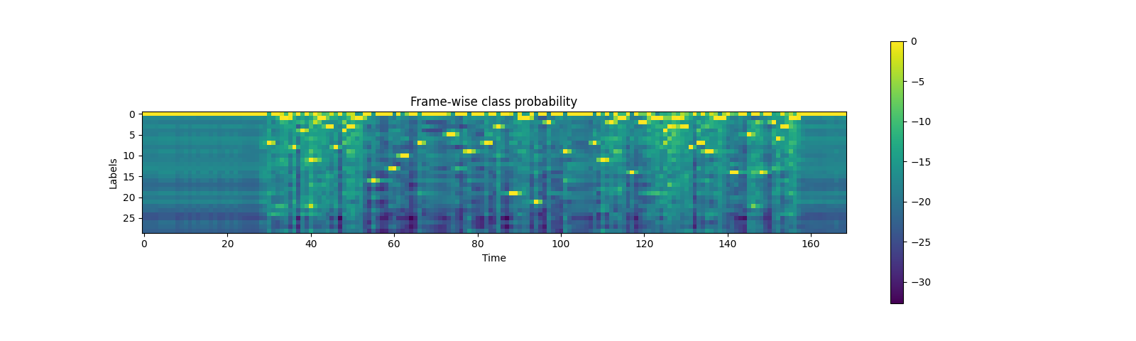
('-', '|', 'E', 'T', 'A', 'O', 'N', 'I', 'H', 'S', 'R', 'D', 'L', 'U', 'M', 'W', 'C', 'F', 'G', 'Y', 'P', 'B', 'V', 'K', "'", 'X', 'J', 'Q', 'Z')
生成对齐概率(网格)
从发射矩阵出发,接下来我们生成格状图(trellis),它表示在每一时间帧上出现转录标签的概率。
Trellis 是一个具有时间轴和标签轴的二维矩阵。标签轴代表我们正在对齐的转录文本。在下文中,我们使用 \(t\) 表示时间轴的索引,使用 \(j\) 表示标签轴的索引。\(c_j\) 表示标签索引为 \(j\) 处的标签。
为了生成时间步 \(t+1\) 的概率,我们查看来自时间步 \(t\) 的格网以及时间步 \(t+1\) 的发射概率。有两条路径可以到达带有标签 \(c_{j+1}\) 的时间步 \(t+1\)。第一种情况是,在 \(t\) 时刻标签为 \(c_{j+1}\),且从 \(t\) 到 \(t+1\) 期间标签未发生变化。另一种情况是,在 \(t\) 时刻标签为 \(c_j\),并在 \(t+1\) 时刻转换到了下一个标签 \(c_{j+1}\)。
下图说明了这一转变。
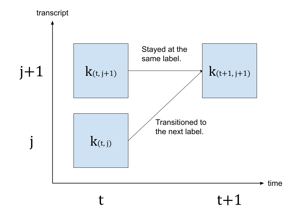
由于我们要寻找最可能的状态转移,因此我们选择概率更高的路径作为 \(k_{(t+1, j+1)}\) 的值,即
\(k_{(t+1, j+1)} = max( k_{(t, j)} p(t+1, c_{j+1}), k_{(t, j+1)} p(t+1, repeat) )\)
其中 \(k\) 代表网格矩阵,而 \(p(t, c_j)\) 代表时间步 \(t\) 处标签 \(c_j\) 的概率。 \(repeat\) 代表来自 CTC 公式的空白标记。(有关 CTC 算法的详细信息,请参阅《使用 CTC 进行序列建模》 [distill.pub])
transcript = "I|HAD|THAT|CURIOSITY|BESIDE|ME|AT|THIS|MOMENT"
dictionary = {c: i for i, c in enumerate(labels)}

tokens = [dictionary[c] for c in transcript]
print(list(zip(transcript, tokens)))


def get_trellis(emission, tokens, blank_id=0):
    num_frame = emission.size(0)
    num_tokens = len(tokens)

    # Trellis has extra diemsions for both time axis and tokens.
    # The extra dim for tokens represents <SoS> (start-of-sentence)
    # The extra dim for time axis is for simplification of the code.
    trellis = torch.empty((num_frame + 1, num_tokens + 1))
    trellis[0, 0] = 0
    trellis[1:, 0] = torch.cumsum(emission[:, 0], 0)
    trellis[0, -num_tokens:] = -float("inf")
    trellis[-num_tokens:, 0] = float("inf")

    for t in range(num_frame):
        trellis[t + 1, 1:] = torch.maximum(
            # Score for staying at the same token
            trellis[t, 1:] + emission[t, blank_id],
            # Score for changing to the next token
            trellis[t, :-1] + emission[t, tokens],
        )
    return trellis


trellis = get_trellis(emission, tokens)
[('I', 7), ('|', 1), ('H', 8), ('A', 4), ('D', 11), ('|', 1), ('T', 3), ('H', 8), ('A', 4), ('T', 3), ('|', 1), ('C', 16), ('U', 13), ('R', 10), ('I', 7), ('O', 5), ('S', 9), ('I', 7), ('T', 3), ('Y', 19), ('|', 1), ('B', 21), ('E', 2), ('S', 9), ('I', 7), ('D', 11), ('E', 2), ('|', 1), ('M', 14), ('E', 2), ('|', 1), ('A', 4), ('T', 3), ('|', 1), ('T', 3), ('H', 8), ('I', 7), ('S', 9), ('|', 1), ('M', 14), ('O', 5), ('M', 14), ('E', 2), ('N', 6), ('T', 3)]
可视化
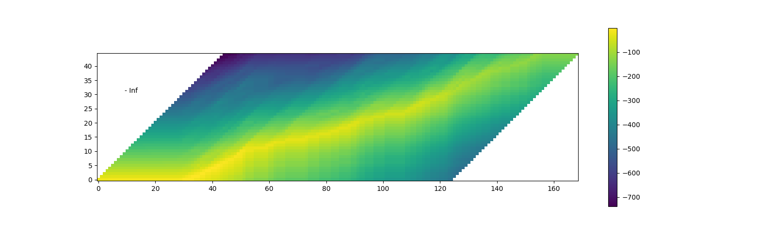
在上述可视化图中,我们可以看到一条高概率轨迹沿矩阵对角线穿过。
查找最可能的路径(回溯)
一旦生成网格,我们将沿着高概率元素对其进行遍历。
我们将从具有最高概率的时间步的最后一个标签索引开始,然后,我们逆时间遍历,根据后转换概率选择停留 (\(c_j \rightarrow c_j\)) 或转换 (\(c_j \rightarrow c_{j+1}\)),基于后转换概率 \(k_{t, j} p(t+1, c_{j+1})\) 或 \(k_{t, j+1} p(t+1, repeat)\)。
当标签到达起始位置时,过渡即完成。
Trellis 矩阵用于路径搜索,但对于每个片段的最终概率,我们采用来自发射矩阵的逐帧概率。
@dataclass
class Point:
    token_index: int
    time_index: int
    score: float


def backtrack(trellis, emission, tokens, blank_id=0):
    # Note:
    # j and t are indices for trellis, which has extra dimensions
    # for time and tokens at the beginning.
    # When referring to time frame index `T` in trellis,
    # the corresponding index in emission is `T-1`.
    # Similarly, when referring to token index `J` in trellis,
    # the corresponding index in transcript is `J-1`.
    j = trellis.size(1) - 1
    t_start = torch.argmax(trellis[:, j]).item()

    path = []
    for t in range(t_start, 0, -1):
        # 1. Figure out if the current position was stay or change
        # Note (again):
        # `emission[J-1]` is the emission at time frame `J` of trellis dimension.
        # Score for token staying the same from time frame J-1 to T.
        stayed = trellis[t - 1, j] + emission[t - 1, blank_id]
        # Score for token changing from C-1 at T-1 to J at T.
        changed = trellis[t - 1, j - 1] + emission[t - 1, tokens[j - 1]]

        # 2. Store the path with frame-wise probability.
        prob = emission[t - 1, tokens[j - 1] if changed > stayed else 0].exp().item()
        # Return token index and time index in non-trellis coordinate.
        path.append(Point(j - 1, t - 1, prob))

        # 3. Update the token
        if changed > stayed:
            j -= 1
            if j == 0:
                break
    else:
        raise ValueError("Failed to align")
    return path[::-1]


path = backtrack(trellis, emission, tokens)
for p in path:
    print(p)
Point(token_index=0, time_index=30, score=0.9999842643737793)
Point(token_index=0, time_index=31, score=0.9846922159194946)
Point(token_index=0, time_index=32, score=0.9999706745147705)
Point(token_index=0, time_index=33, score=0.15398240089416504)
Point(token_index=1, time_index=34, score=0.9999173879623413)
Point(token_index=1, time_index=35, score=0.6080460548400879)
Point(token_index=2, time_index=36, score=0.9997721314430237)
Point(token_index=2, time_index=37, score=0.9997130036354065)
Point(token_index=3, time_index=38, score=0.9999358654022217)
Point(token_index=3, time_index=39, score=0.9861565828323364)
Point(token_index=4, time_index=40, score=0.923857569694519)
Point(token_index=4, time_index=41, score=0.9257341027259827)
Point(token_index=4, time_index=42, score=0.015660513192415237)
Point(token_index=5, time_index=43, score=0.9998378753662109)
Point(token_index=6, time_index=44, score=0.9988443851470947)
Point(token_index=6, time_index=45, score=0.10142531245946884)
Point(token_index=7, time_index=46, score=0.9999427795410156)
Point(token_index=7, time_index=47, score=0.9999943971633911)
Point(token_index=8, time_index=48, score=0.9979603290557861)
Point(token_index=8, time_index=49, score=0.036034904420375824)
Point(token_index=8, time_index=50, score=0.06163628771901131)
Point(token_index=9, time_index=51, score=4.334864570409991e-05)
Point(token_index=10, time_index=52, score=0.9999799728393555)
Point(token_index=10, time_index=53, score=0.996708869934082)
Point(token_index=10, time_index=54, score=0.9999256134033203)
Point(token_index=11, time_index=55, score=0.9999983310699463)
Point(token_index=11, time_index=56, score=0.9990686774253845)
Point(token_index=11, time_index=57, score=0.9999996423721313)
Point(token_index=11, time_index=58, score=0.9999996423721313)
Point(token_index=11, time_index=59, score=0.845734179019928)
Point(token_index=12, time_index=60, score=0.9999996423721313)
Point(token_index=12, time_index=61, score=0.9996010661125183)
Point(token_index=13, time_index=62, score=0.999998927116394)
Point(token_index=13, time_index=63, score=0.0035242538433521986)
Point(token_index=13, time_index=64, score=1.0)
Point(token_index=13, time_index=65, score=1.0)
Point(token_index=14, time_index=66, score=0.9999915361404419)
Point(token_index=14, time_index=67, score=0.9971554279327393)
Point(token_index=14, time_index=68, score=0.9999990463256836)
Point(token_index=14, time_index=69, score=0.9999992847442627)
Point(token_index=14, time_index=70, score=0.9999997615814209)
Point(token_index=14, time_index=71, score=0.9999998807907104)
Point(token_index=14, time_index=72, score=0.9999880790710449)
Point(token_index=14, time_index=73, score=0.01142667606472969)
Point(token_index=15, time_index=74, score=0.9999977350234985)
Point(token_index=15, time_index=75, score=0.9996134042739868)
Point(token_index=15, time_index=76, score=0.999998927116394)
Point(token_index=15, time_index=77, score=0.9727587103843689)
Point(token_index=16, time_index=78, score=0.999998927116394)
Point(token_index=16, time_index=79, score=0.9949321150779724)
Point(token_index=16, time_index=80, score=0.999998927116394)
Point(token_index=16, time_index=81, score=0.9999121427536011)
Point(token_index=17, time_index=82, score=0.9999774694442749)
Point(token_index=17, time_index=83, score=0.657580554485321)
Point(token_index=17, time_index=84, score=0.9984301924705505)
Point(token_index=18, time_index=85, score=0.9999876022338867)
Point(token_index=18, time_index=86, score=0.9993745684623718)
Point(token_index=18, time_index=87, score=0.9999988079071045)
Point(token_index=18, time_index=88, score=0.10423555970191956)
Point(token_index=19, time_index=89, score=0.9999969005584717)
Point(token_index=19, time_index=90, score=0.39787012338638306)
Point(token_index=20, time_index=91, score=0.9999932050704956)
Point(token_index=20, time_index=92, score=1.6991340316963033e-06)
Point(token_index=20, time_index=93, score=0.9861343502998352)
Point(token_index=21, time_index=94, score=0.9999960660934448)
Point(token_index=21, time_index=95, score=0.9992730021476746)
Point(token_index=21, time_index=96, score=0.9993410706520081)
Point(token_index=22, time_index=97, score=0.9999983310699463)
Point(token_index=22, time_index=98, score=0.9999971389770508)
Point(token_index=22, time_index=99, score=0.9999998807907104)
Point(token_index=22, time_index=100, score=0.9999995231628418)
Point(token_index=23, time_index=101, score=0.9999732971191406)
Point(token_index=23, time_index=102, score=0.9983224272727966)
Point(token_index=23, time_index=103, score=0.9999991655349731)
Point(token_index=23, time_index=104, score=0.9999996423721313)
Point(token_index=23, time_index=105, score=0.9999998807907104)
Point(token_index=23, time_index=106, score=1.0)
Point(token_index=23, time_index=107, score=0.9998630285263062)
Point(token_index=24, time_index=108, score=0.9999980926513672)
Point(token_index=24, time_index=109, score=0.9988585710525513)
Point(token_index=25, time_index=110, score=0.9999798536300659)
Point(token_index=25, time_index=111, score=0.857322633266449)
Point(token_index=26, time_index=112, score=0.9999847412109375)
Point(token_index=26, time_index=113, score=0.987025260925293)
Point(token_index=26, time_index=114, score=1.9046619854634628e-05)
Point(token_index=27, time_index=115, score=0.9999794960021973)
Point(token_index=27, time_index=116, score=0.9998254776000977)
Point(token_index=28, time_index=117, score=0.9999990463256836)
Point(token_index=28, time_index=118, score=0.9999732971191406)
Point(token_index=28, time_index=119, score=0.000900460931006819)
Point(token_index=29, time_index=120, score=0.9993478655815125)
Point(token_index=29, time_index=121, score=0.9975457787513733)
Point(token_index=29, time_index=122, score=0.00030494449310936034)
Point(token_index=30, time_index=123, score=0.9999344348907471)
Point(token_index=30, time_index=124, score=6.079339982534293e-06)
Point(token_index=31, time_index=125, score=0.9833164811134338)
Point(token_index=32, time_index=126, score=0.9974580407142639)
Point(token_index=32, time_index=127, score=0.0008237393340095878)
Point(token_index=33, time_index=128, score=0.9965153932571411)
Point(token_index=33, time_index=129, score=0.017462942749261856)
Point(token_index=34, time_index=130, score=0.9989171028137207)
Point(token_index=35, time_index=131, score=0.9999697208404541)
Point(token_index=35, time_index=132, score=0.9999842643737793)
Point(token_index=36, time_index=133, score=0.9997640252113342)
Point(token_index=36, time_index=134, score=0.5097429752349854)
Point(token_index=37, time_index=135, score=0.9998301267623901)
Point(token_index=37, time_index=136, score=0.08522891998291016)
Point(token_index=37, time_index=137, score=0.004074938595294952)
Point(token_index=38, time_index=138, score=0.9999815225601196)
Point(token_index=38, time_index=139, score=0.012054883874952793)
Point(token_index=38, time_index=140, score=0.9999980926513672)
Point(token_index=38, time_index=141, score=0.0005777245969511569)
Point(token_index=39, time_index=142, score=0.9999066591262817)
Point(token_index=39, time_index=143, score=0.9999960660934448)
Point(token_index=39, time_index=144, score=0.9999980926513672)
Point(token_index=40, time_index=145, score=0.9999916553497314)
Point(token_index=40, time_index=146, score=0.9971165657043457)
Point(token_index=40, time_index=147, score=0.9981800317764282)
Point(token_index=41, time_index=148, score=0.9999310970306396)
Point(token_index=41, time_index=149, score=0.9879499673843384)
Point(token_index=41, time_index=150, score=0.9997627139091492)
Point(token_index=42, time_index=151, score=0.9999535083770752)
Point(token_index=43, time_index=152, score=0.9999715089797974)
Point(token_index=44, time_index=153, score=0.681148886680603)
可视化
def plot_trellis_with_path(trellis, path):
    # To plot trellis with path, we take advantage of 'nan' value
    trellis_with_path = trellis.clone()
    for _, p in enumerate(path):
        trellis_with_path[p.time_index, p.token_index] = float("nan")
    plt.imshow(trellis_with_path[1:, 1:].T, origin="lower")


plot_trellis_with_path(trellis, path)
plt.title("The path found by backtracking")
plt.show()
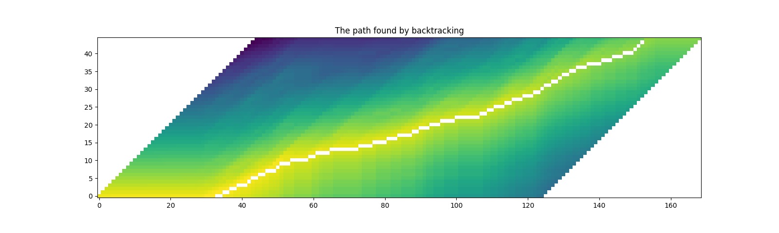
看起来不错。现在这条路径包含相同标签的重复项,因此让我们将它们合并,使其更接近原始转录稿。
在合并多个路径点时,我们直接对合并后的片段取平均概率。
# Merge the labels
@dataclass
class Segment:
    label: str
    start: int
    end: int
    score: float

    def __repr__(self):
        return f"{self.label}\t({self.score:4.2f}): [{self.start:5d}, {self.end:5d})"

    @property
    def length(self):
        return self.end - self.start


def merge_repeats(path):
    i1, i2 = 0, 0
    segments = []
    while i1 < len(path):
        while i2 < len(path) and path[i1].token_index == path[i2].token_index:
            i2 += 1
        score = sum(path[k].score for k in range(i1, i2)) / (i2 - i1)
        segments.append(
            Segment(
                transcript[path[i1].token_index],
                path[i1].time_index,
                path[i2 - 1].time_index + 1,
                score,
            )
        )
        i1 = i2
    return segments


segments = merge_repeats(path)
for seg in segments:
    print(seg)
I       (0.78): [   30,    34)
|       (0.80): [   34,    36)
H       (1.00): [   36,    38)
A       (0.99): [   38,    40)
D       (0.62): [   40,    43)
|       (1.00): [   43,    44)
T       (0.55): [   44,    46)
H       (1.00): [   46,    48)
A       (0.37): [   48,    51)
T       (0.00): [   51,    52)
|       (1.00): [   52,    55)
C       (0.97): [   55,    60)
U       (1.00): [   60,    62)
R       (0.75): [   62,    66)
I       (0.88): [   66,    74)
O       (0.99): [   74,    78)
S       (1.00): [   78,    82)
I       (0.89): [   82,    85)
T       (0.78): [   85,    89)
Y       (0.70): [   89,    91)
|       (0.66): [   91,    94)
B       (1.00): [   94,    97)
E       (1.00): [   97,   101)
S       (1.00): [  101,   108)
I       (1.00): [  108,   110)
D       (0.93): [  110,   112)
E       (0.66): [  112,   115)
|       (1.00): [  115,   117)
M       (0.67): [  117,   120)
E       (0.67): [  120,   123)
|       (0.50): [  123,   125)
A       (0.98): [  125,   126)
T       (0.50): [  126,   128)
|       (0.51): [  128,   130)
T       (1.00): [  130,   131)
H       (1.00): [  131,   133)
I       (0.75): [  133,   135)
S       (0.36): [  135,   138)
|       (0.50): [  138,   142)
M       (1.00): [  142,   145)
O       (1.00): [  145,   148)
M       (1.00): [  148,   151)
E       (1.00): [  151,   152)
N       (1.00): [  152,   153)
T       (0.68): [  153,   154)
可视化
def plot_trellis_with_segments(trellis, segments, transcript):
    # To plot trellis with path, we take advantage of 'nan' value
    trellis_with_path = trellis.clone()
    for i, seg in enumerate(segments):
        if seg.label != "|":
            trellis_with_path[seg.start + 1 : seg.end + 1, i + 1] = float("nan")

    fig, [ax1, ax2] = plt.subplots(2, 1, figsize=(16, 9.5))
    ax1.set_title("Path, label and probability for each label")
    ax1.imshow(trellis_with_path.T, origin="lower")
    ax1.set_xticks([])

    for i, seg in enumerate(segments):
        if seg.label != "|":
            ax1.annotate(seg.label, (seg.start + 0.7, i + 0.3), weight="bold")
            ax1.annotate(f"{seg.score:.2f}", (seg.start - 0.3, i + 4.3))

    ax2.set_title("Label probability with and without repetation")
    xs, hs, ws = [], [], []
    for seg in segments:
        if seg.label != "|":
            xs.append((seg.end + seg.start) / 2 + 0.4)
            hs.append(seg.score)
            ws.append(seg.end - seg.start)
            ax2.annotate(seg.label, (seg.start + 0.8, -0.07), weight="bold")
    ax2.bar(xs, hs, width=ws, color="gray", alpha=0.5, edgecolor="black")

    xs, hs = [], []
    for p in path:
        label = transcript[p.token_index]
        if label != "|":
            xs.append(p.time_index + 1)
            hs.append(p.score)

    ax2.bar(xs, hs, width=0.5, alpha=0.5)
    ax2.axhline(0, color="black")
    ax2.set_xlim(ax1.get_xlim())
    ax2.set_ylim(-0.1, 1.1)


plot_trellis_with_segments(trellis, segments, transcript)
plt.tight_layout()
plt.show()
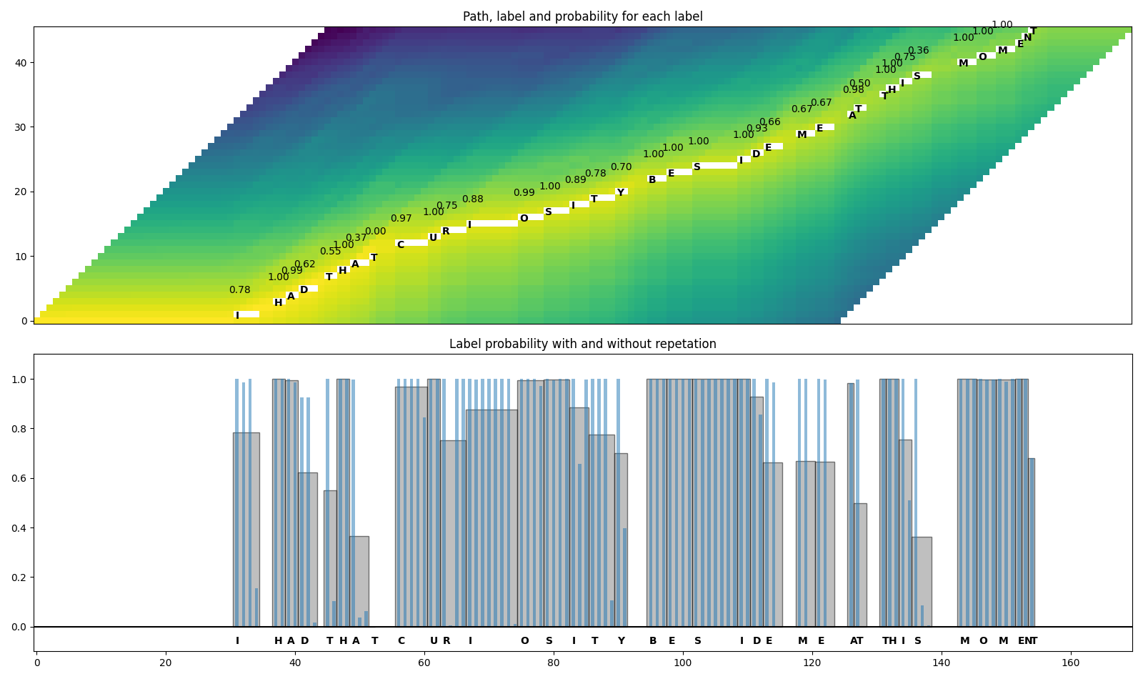
看起来不错。现在让我们合并单词。Wav2Vec2 模型使用 '|'
作为词边界,因此我们在每次出现
'|'之前合并片段。
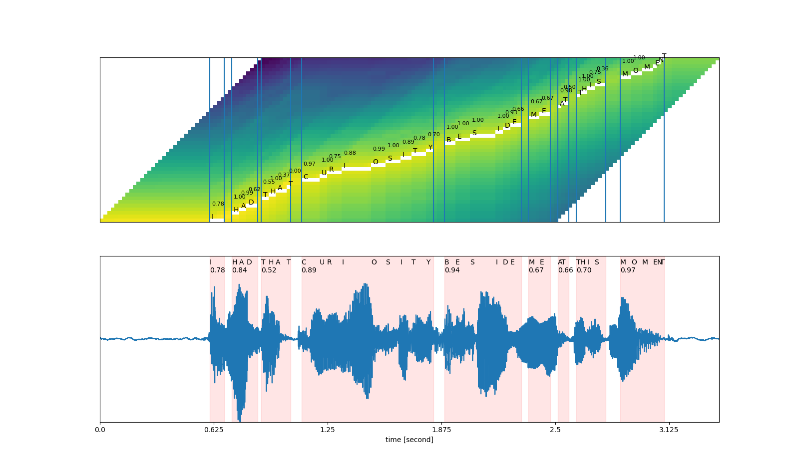
最后,我们将原始音频分割为分段音频,并聆听这些片段以验证分割是否正确。
# Merge words
def merge_words(segments, separator="|"):
    words = []
    i1, i2 = 0, 0
    while i1 < len(segments):
        if i2 >= len(segments) or segments[i2].label == separator:
            if i1 != i2:
                segs = segments[i1:i2]
                word = "".join([seg.label for seg in segs])
                score = sum(seg.score * seg.length for seg in segs) / sum(seg.length for seg in segs)
                words.append(Segment(word, segments[i1].start, segments[i2 - 1].end, score))
            i1 = i2 + 1
            i2 = i1
        else:
            i2 += 1
    return words


word_segments = merge_words(segments)
for word in word_segments:
    print(word)
I       (0.78): [   30,    34)
HAD     (0.84): [   36,    43)
THAT    (0.52): [   44,    52)
CURIOSITY       (0.89): [   55,    91)
BESIDE  (0.94): [   94,   115)
ME      (0.67): [  117,   123)
AT      (0.66): [  125,   128)
THIS    (0.70): [  130,   138)
MOMENT  (0.97): [  142,   154)
可视化
def plot_alignments(trellis, segments, word_segments, waveform):
    trellis_with_path = trellis.clone()
    for i, seg in enumerate(segments):
        if seg.label != "|":
            trellis_with_path[seg.start + 1 : seg.end + 1, i + 1] = float("nan")

    fig, [ax1, ax2] = plt.subplots(2, 1, figsize=(16, 9.5))

    ax1.imshow(trellis_with_path[1:, 1:].T, origin="lower")
    ax1.set_xticks([])
    ax1.set_yticks([])

    for word in word_segments:
        ax1.axvline(word.start - 0.5)
        ax1.axvline(word.end - 0.5)

    for i, seg in enumerate(segments):
        if seg.label != "|":
            ax1.annotate(seg.label, (seg.start, i + 0.3))
            ax1.annotate(f"{seg.score:.2f}", (seg.start, i + 4), fontsize=8)

    # The original waveform
    ratio = waveform.size(0) / (trellis.size(0) - 1)
    ax2.plot(waveform)
    for word in word_segments:
        x0 = ratio * word.start
        x1 = ratio * word.end
        ax2.axvspan(x0, x1, alpha=0.1, color="red")
        ax2.annotate(f"{word.score:.2f}", (x0, 0.8))

    for seg in segments:
        if seg.label != "|":
            ax2.annotate(seg.label, (seg.start * ratio, 0.9))
    xticks = ax2.get_xticks()
    plt.xticks(xticks, xticks / bundle.sample_rate)
    ax2.set_xlabel("time [second]")
    ax2.set_yticks([])
    ax2.set_ylim(-1.0, 1.0)
    ax2.set_xlim(0, waveform.size(-1))


plot_alignments(
    trellis,
    segments,
    word_segments,
    waveform[0],
)
plt.show()
# A trick to embed the resulting audio to the generated file.
# `IPython.display.Audio` has to be the last call in a cell,
# and there should be only one call par cell.
def display_segment(i):
    ratio = waveform.size(1) / (trellis.size(0) - 1)
    word = word_segments[i]
    x0 = int(ratio * word.start)
    x1 = int(ratio * word.end)
    print(f"{word.label} ({word.score:.2f}): {x0 / bundle.sample_rate:.3f} - {x1 / bundle.sample_rate:.3f} sec")
    segment = waveform[:, x0:x1]
    return IPython.display.Audio(segment.numpy(), rate=bundle.sample_rate)
# Generate the audio for each segment
print(transcript)
IPython.display.Audio(SPEECH_FILE)
I|HAD|THAT|CURIOSITY|BESIDE|ME|AT|THIS|MOMENT
display_segment(0)
I (0.78): 0.604 - 0.684 sec
display_segment(1)
HAD (0.84): 0.724 - 0.865 sec
display_segment(2)
THAT (0.52): 0.885 - 1.046 sec
display_segment(3)
CURIOSITY (0.89): 1.107 - 1.831 sec
display_segment(4)
BESIDE (0.94): 1.891 - 2.314 sec
display_segment(5)
ME (0.67): 2.354 - 2.474 sec
display_segment(6)
AT (0.66): 2.515 - 2.575 sec
display_segment(7)
THIS (0.70): 2.615 - 2.776 sec
display_segment(8)
MOMENT (0.97): 2.857 - 3.098 sec
结论
在本教程中,我们探讨了如何使用 torchaudio 的 Wav2Vec2 模型执行 CTC 分割以实现强制对齐。
脚本的总运行时间: ( 0 分钟 3.182 秒)