注意

点击这里下载完整示例代码

使用 Tacotron2 进行文本转语音¶

import IPython
import matplotlib
import matplotlib.pyplot as plt

概述¶

本教程展示了如何使用 torchaudio 中预训练的 Tacotron2 构建文本转语音流程。

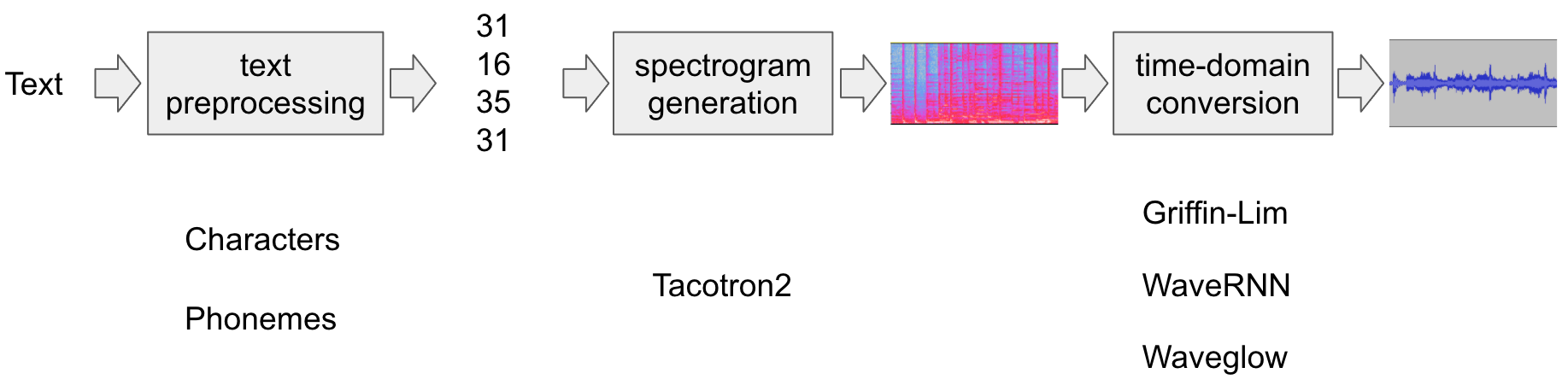
文本转语音流程如下：

文本预处理

首先，输入文本被编码为符号列表。在本教程中，我们将使用英文字符和音素作为符号。
频谱图生成

从编码文本生成频谱图。我们使用 Tacotron2 模型来完成此操作。
时域转换

最后一步是将语谱图转换为波形。从语谱图生成语音的过程也称为声码器（Vocoder）。在本教程中，我们使用了三种不同的声码器： WaveRNN、 Griffin-Lim 以及 Nvidia 的 WaveGlow。

下图展示了整个流程。

https://download.pytorch.org/torchaudio/tutorial-assets/tacotron2_tts_pipeline.png

所有相关组件都打包在 torchaudio.pipelines.Tacotron2TTSBundle() 中，但本教程也将涵盖其背后的处理过程。

准备¶

首先，我们安装必要的依赖项。除了 torchaudio，还需要 DeepPhonemizer 来执行基于音素的编码。

# When running this example in notebook, install DeepPhonemizer
# !pip3 install deep_phonemizer

import torch
import torchaudio

matplotlib.rcParams["figure.figsize"] = [16.0, 4.8]

torch.random.manual_seed(0)
device = "cuda" if torch.cuda.is_available() else "cpu"

print(torch.__version__)
print(torchaudio.__version__)
print(device)

Out:

1.12.0
0.12.0
cpu

文本处理¶

基于字符的编码¶

在本节中，我们将介绍基于字符的编码是如何工作的。

由于预训练的 Tacotron2 模型需要特定的符号表集，因此提供了与 torchaudio 中相同的功能。本节主要用于解释编码的基础知识。

首先，我们定义符号集。例如，我们可以使用 '_-!\'(),.:;? abcdefghijklmnopqrstuvwxyz'。然后，我们将输入文本中的每个字符映射到表中对应符号的索引。

以下是此类处理的一个示例。在该示例中，表中未出现的符号将被忽略。

symbols = "_-!'(),.:;? abcdefghijklmnopqrstuvwxyz"
look_up = {s: i for i, s in enumerate(symbols)}
symbols = set(symbols)


def text_to_sequence(text):
    text = text.lower()
    return [look_up[s] for s in text if s in symbols]


text = "Hello world! Text to speech!"
print(text_to_sequence(text))

Out:

[19, 16, 23, 23, 26, 11, 34, 26, 29, 23, 15, 2, 11, 31, 16, 35, 31, 11, 31, 26, 11, 30, 27, 16, 16, 14, 19, 2]

如上所述，符号表和索引必须与预训练的 Tacotron2 模型所期望的一致。torchaudio 提供了该转换以及预训练模型。例如，您可以实例化并使用此类转换，如下所示。

processor = torchaudio.pipelines.TACOTRON2_WAVERNN_CHAR_LJSPEECH.get_text_processor()

text = "Hello world! Text to speech!"
processed, lengths = processor(text)

print(processed)
print(lengths)

Out:

tensor([[19, 16, 23, 23, 26, 11, 34, 26, 29, 23, 15,  2, 11, 31, 16, 35, 31, 11,
         31, 26, 11, 30, 27, 16, 16, 14, 19,  2]])
tensor([28], dtype=torch.int32)

The processor 对象接受文本或文本列表作为输入。当提供文本列表时，返回的 lengths 变量表示输出批次中每个处理过的标记的有效长度。

中间表示可按以下方式检索。

print([processor.tokens[i] for i in processed[0, : lengths[0]]])

Out:

['h', 'e', 'l', 'l', 'o', ' ', 'w', 'o', 'r', 'l', 'd', '!', ' ', 't', 'e', 'x', 't', ' ', 't', 'o', ' ', 's', 'p', 'e', 'e', 'c', 'h', '!']

基于音素的编码¶

基于音素的编码与基于字符的编码类似，但它使用基于音素的符号表和一个 G2P（字形到音素）模型。

G2P 模型的细节超出了本教程的范围，我们仅查看转换后的效果。

与基于字符的编码情况类似，编码过程应与预训练的 Tacotron2 模型所训练的内容相匹配。 torchaudio 提供了一个用于创建该过程的接口。

以下代码说明了如何创建和使用该流程。在后台，使用 DeepPhonemizer 包创建一个 G2P 模型，并获取 DeepPhonemizer 的作者发布的预训练权重。

bundle = torchaudio.pipelines.TACOTRON2_WAVERNN_PHONE_LJSPEECH

processor = bundle.get_text_processor()

text = "Hello world! Text to speech!"
with torch.inference_mode():
    processed, lengths = processor(text)

print(processed)
print(lengths)

Out:

  0%|          | 0.00/63.6M [00:00<?, ?B/s]
  0%|          | 56.0k/63.6M [00:00<03:29, 318kB/s]
  0%|          | 192k/63.6M [00:00<01:53, 584kB/s]
  1%|1         | 872k/63.6M [00:00<00:31, 2.07MB/s]
  5%|5         | 3.21M/63.6M [00:00<00:09, 6.65MB/s]
  9%|8         | 5.73M/63.6M [00:00<00:06, 9.50MB/s]
 14%|#3        | 8.73M/63.6M [00:01<00:04, 12.2MB/s]
 18%|#8        | 11.7M/63.6M [00:01<00:03, 13.9MB/s]
 23%|##3       | 14.7M/63.6M [00:01<00:03, 15.0MB/s]
 28%|##7       | 17.7M/63.6M [00:01<00:03, 15.7MB/s]
 33%|###2      | 20.7M/63.6M [00:01<00:02, 16.2MB/s]
 37%|###7      | 23.7M/63.6M [00:01<00:02, 16.5MB/s]
 42%|####1     | 26.7M/63.6M [00:02<00:02, 16.8MB/s]
 47%|####6     | 29.7M/63.6M [00:02<00:02, 17.0MB/s]
 51%|#####1    | 32.6M/63.6M [00:02<00:01, 19.5MB/s]
 54%|#####4    | 34.6M/63.6M [00:02<00:01, 17.0MB/s]
 58%|#####8    | 37.2M/63.6M [00:02<00:01, 16.5MB/s]
 63%|######3   | 40.2M/63.6M [00:02<00:01, 16.8MB/s]
 68%|######7   | 43.2M/63.6M [00:03<00:01, 17.0MB/s]
 72%|#######1  | 45.7M/63.6M [00:03<00:00, 19.0MB/s]
 75%|#######4  | 47.7M/63.6M [00:03<00:01, 16.5MB/s]
 80%|#######9  | 50.7M/63.6M [00:03<00:00, 16.8MB/s]
 84%|########4 | 53.7M/63.6M [00:03<00:00, 16.9MB/s]
 89%|########9 | 56.7M/63.6M [00:03<00:00, 17.2MB/s]
 92%|#########2| 58.8M/63.6M [00:04<00:00, 18.1MB/s]
 96%|#########6| 61.2M/63.6M [00:04<00:00, 16.9MB/s]
100%|##########| 63.6M/63.6M [00:04<00:00, 15.3MB/s]
tensor([[54, 20, 65, 69, 11, 92, 44, 65, 38,  2, 11, 81, 40, 64, 79, 81, 11, 81,
         20, 11, 79, 77, 59, 37,  2]])
tensor([25], dtype=torch.int32)

请注意，编码后的值与基于字符的编码示例不同。

中间表示形式如下所示。

print([processor.tokens[i] for i in processed[0, : lengths[0]]])

Out:

['HH', 'AH', 'L', 'OW', ' ', 'W', 'ER', 'L', 'D', '!', ' ', 'T', 'EH', 'K', 'S', 'T', ' ', 'T', 'AH', ' ', 'S', 'P', 'IY', 'CH', '!']

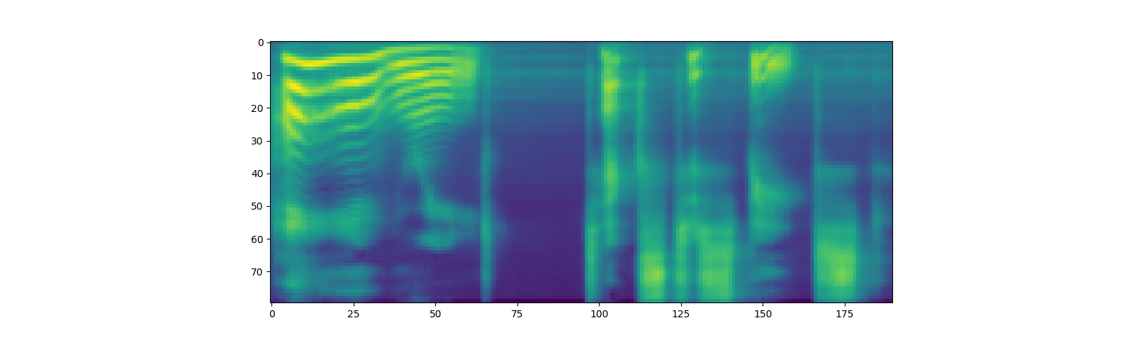
频谱图生成¶

Tacotron2 是我们用来从编码文本生成频谱图的模型。有关该模型的详细信息，请参阅论文。

使用预训练权重实例化 Tacotron2 模型非常简单，但请注意，输入到 Tacotron2 模型的数据需要经过匹配文本处理器的处理。

torchaudio.pipelines.Tacotron2TTSBundle() 将匹配的模型和处理器捆绑在一起，以便轻松创建流水线。

有关可用的捆绑包及其用法，请参阅 torchaudio.pipelines。

bundle = torchaudio.pipelines.TACOTRON2_WAVERNN_PHONE_LJSPEECH
processor = bundle.get_text_processor()
tacotron2 = bundle.get_tacotron2().to(device)

text = "Hello world! Text to speech!"

with torch.inference_mode():
    processed, lengths = processor(text)
    processed = processed.to(device)
    lengths = lengths.to(device)
    spec, _, _ = tacotron2.infer(processed, lengths)


plt.imshow(spec[0].cpu().detach())

Out:

Downloading: "https://download.pytorch.org/torchaudio/models/tacotron2_english_phonemes_1500_epochs_wavernn_ljspeech.pth" to /root/.cache/torch/hub/checkpoints/tacotron2_english_phonemes_1500_epochs_wavernn_ljspeech.pth

  0%|          | 0.00/107M [00:00<?, ?B/s]
  4%|4         | 4.40M/107M [00:00<00:02, 46.1MB/s]
  8%|8         | 8.80M/107M [00:00<00:02, 45.3MB/s]
 14%|#3        | 15.0M/107M [00:00<00:01, 54.2MB/s]
 20%|##        | 21.7M/107M [00:00<00:01, 60.1MB/s]
 26%|##5       | 27.5M/107M [00:00<00:01, 47.8MB/s]
 32%|###1      | 34.0M/107M [00:00<00:01, 53.8MB/s]
 38%|###8      | 41.2M/107M [00:00<00:01, 60.1MB/s]
 45%|####5     | 48.6M/107M [00:00<00:00, 65.1MB/s]
 52%|#####2    | 56.0M/107M [00:00<00:00, 68.9MB/s]
 58%|#####8    | 62.8M/107M [00:01<00:00, 69.4MB/s]
 65%|######4   | 69.7M/107M [00:01<00:00, 70.3MB/s]
 71%|#######1  | 76.5M/107M [00:01<00:00, 67.5MB/s]
 77%|#######7  | 83.0M/107M [00:01<00:00, 62.2MB/s]
 83%|########2 | 89.2M/107M [00:01<00:00, 59.3MB/s]
 89%|########8 | 95.4M/107M [00:01<00:00, 60.8MB/s]
 94%|#########4| 101M/107M [00:01<00:00, 60.5MB/s]
100%|#########9| 107M/107M [00:01<00:00, 59.8MB/s]
100%|##########| 107M/107M [00:01<00:00, 60.6MB/s]

<matplotlib.image.AxesImage object at 0x7fd8fd4d97f0>

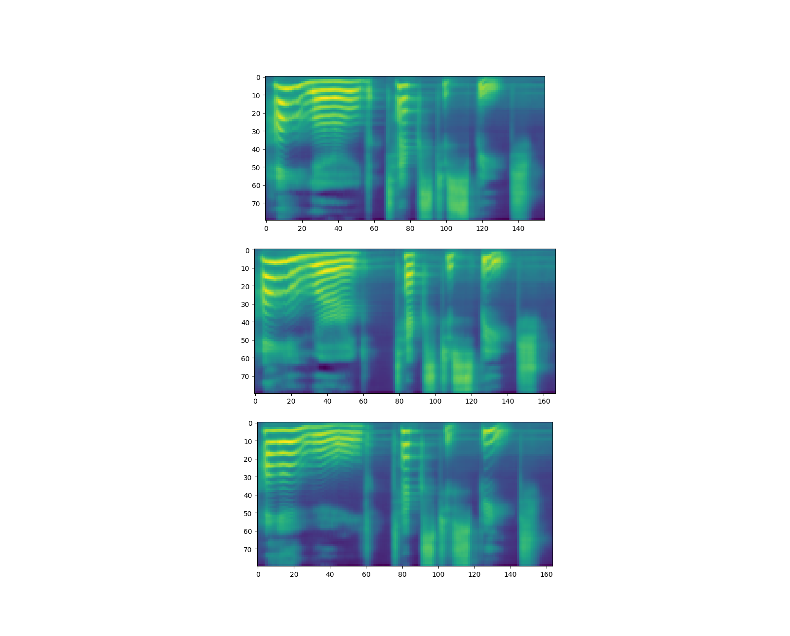
请注意，Tacotron2.infer 方法执行多项式采样，因此生成频谱图的过程会引入随机性。

fig, ax = plt.subplots(3, 1, figsize=(16, 4.3 * 3))
for i in range(3):
    with torch.inference_mode():
        spec, spec_lengths, _ = tacotron2.infer(processed, lengths)
    print(spec[0].shape)
    ax[i].imshow(spec[0].cpu().detach())
plt.show()

Out:

torch.Size([80, 155])
torch.Size([80, 167])
torch.Size([80, 164])

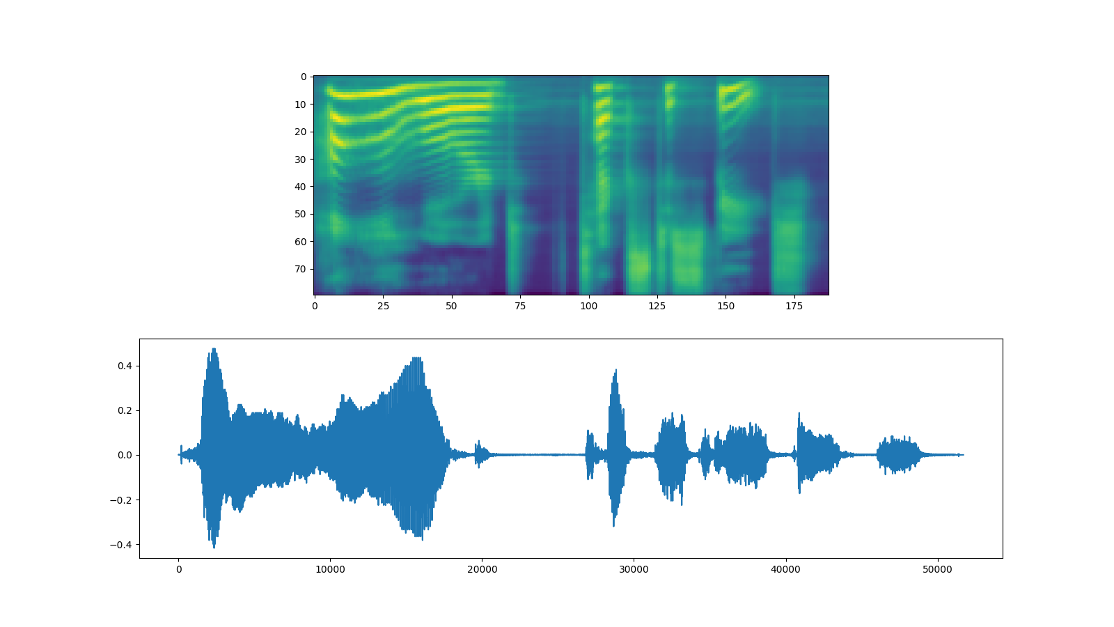
波形生成¶

生成频谱图后，最后一步是从频谱图中恢复波形。

torchaudio 提供基于 GriffinLim 和 WaveRNN 的声码器。

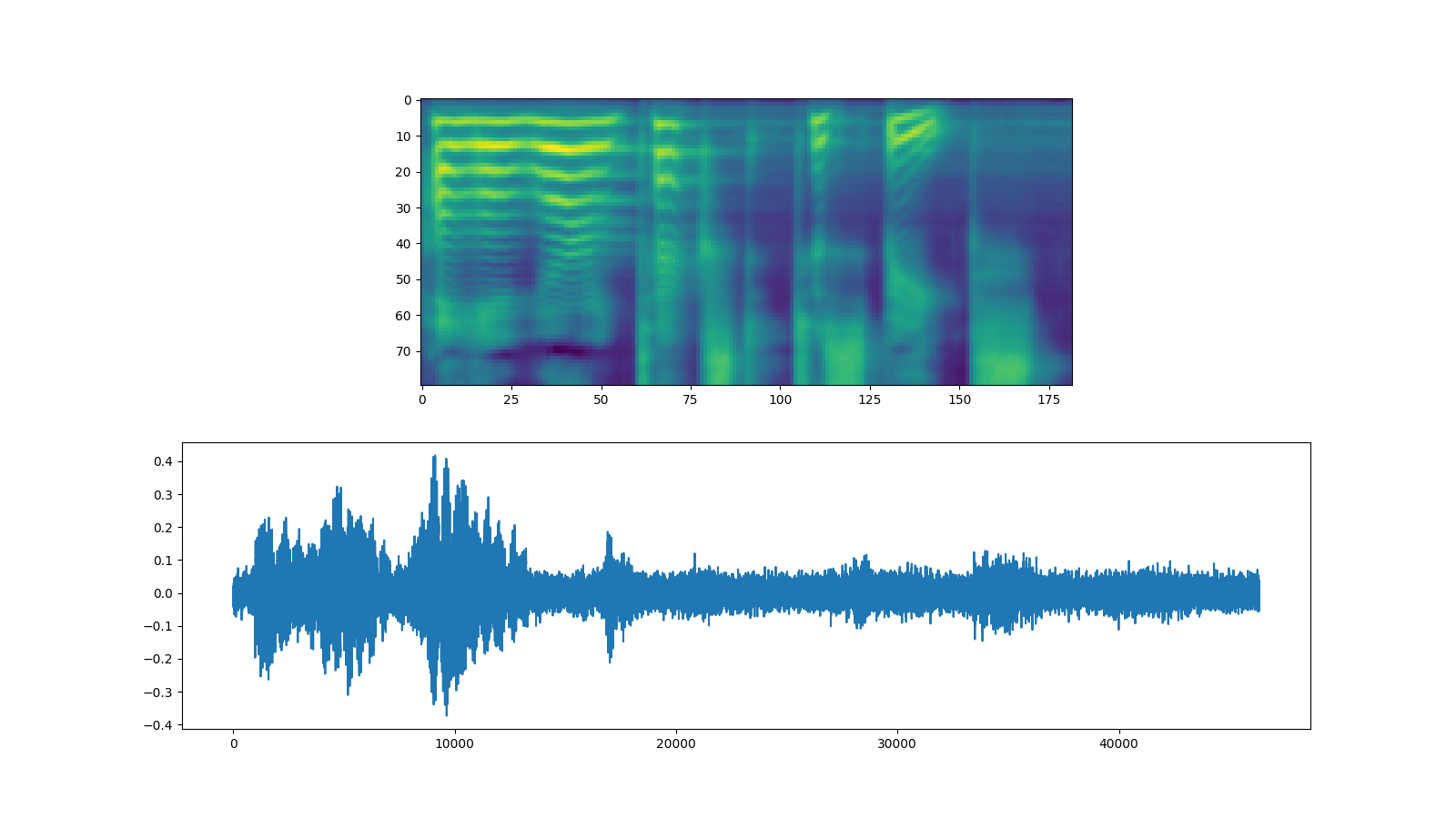
WaveRNN¶

承接上一节，我们可以从同一个捆绑包中实例化匹配的 WaveRNN 模型。

bundle = torchaudio.pipelines.TACOTRON2_WAVERNN_PHONE_LJSPEECH

processor = bundle.get_text_processor()
tacotron2 = bundle.get_tacotron2().to(device)
vocoder = bundle.get_vocoder().to(device)

text = "Hello world! Text to speech!"

with torch.inference_mode():
    processed, lengths = processor(text)
    processed = processed.to(device)
    lengths = lengths.to(device)
    spec, spec_lengths, _ = tacotron2.infer(processed, lengths)
    waveforms, lengths = vocoder(spec, spec_lengths)

fig, [ax1, ax2] = plt.subplots(2, 1, figsize=(16, 9))
ax1.imshow(spec[0].cpu().detach())
ax2.plot(waveforms[0].cpu().detach())

torchaudio.save("_assets/output_wavernn.wav", waveforms[0:1].cpu(), sample_rate=vocoder.sample_rate)
IPython.display.Audio("_assets/output_wavernn.wav")

Out:

Downloading: "https://download.pytorch.org/torchaudio/models/wavernn_10k_epochs_8bits_ljspeech.pth" to /root/.cache/torch/hub/checkpoints/wavernn_10k_epochs_8bits_ljspeech.pth

  0%|          | 0.00/16.7M [00:00<?, ?B/s]
 42%|####1     | 6.98M/16.7M [00:00<00:00, 73.2MB/s]
 84%|########3 | 14.0M/16.7M [00:00<00:00, 72.6MB/s]
100%|##########| 16.7M/16.7M [00:00<00:00, 69.3MB/s]

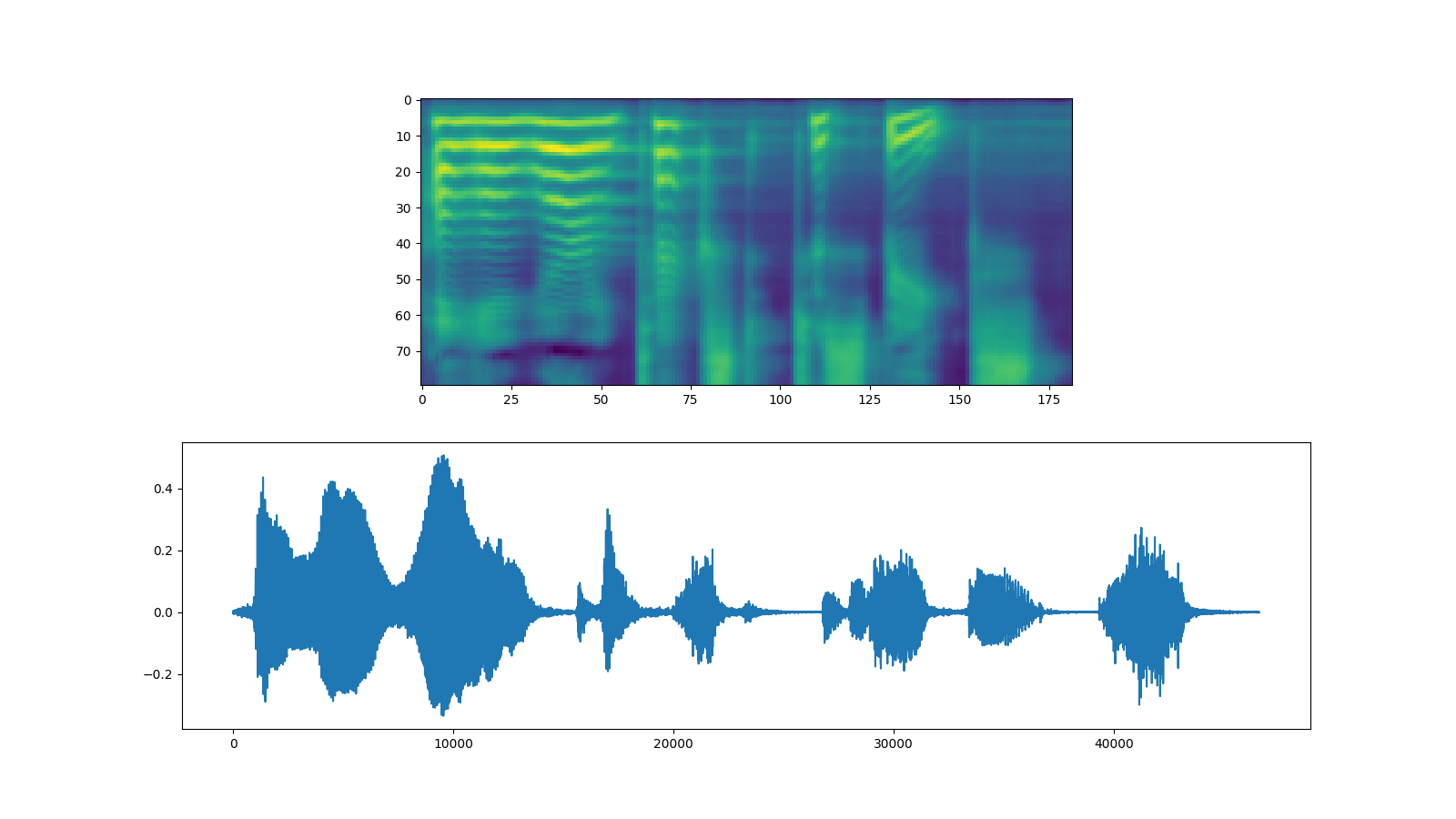
Griffin-Lim¶

使用 Griffin-Lim 声码器与 WaveRNN 相同。您可以使用 get_vocoder 方法实例化声码器对象并传入频谱图。

bundle = torchaudio.pipelines.TACOTRON2_GRIFFINLIM_PHONE_LJSPEECH

processor = bundle.get_text_processor()
tacotron2 = bundle.get_tacotron2().to(device)
vocoder = bundle.get_vocoder().to(device)

with torch.inference_mode():
    processed, lengths = processor(text)
    processed = processed.to(device)
    lengths = lengths.to(device)
    spec, spec_lengths, _ = tacotron2.infer(processed, lengths)
waveforms, lengths = vocoder(spec, spec_lengths)

fig, [ax1, ax2] = plt.subplots(2, 1, figsize=(16, 9))
ax1.imshow(spec[0].cpu().detach())
ax2.plot(waveforms[0].cpu().detach())

torchaudio.save(
    "_assets/output_griffinlim.wav",
    waveforms[0:1].cpu(),
    sample_rate=vocoder.sample_rate,
)
IPython.display.Audio("_assets/output_griffinlim.wav")

Out:

Downloading: "https://download.pytorch.org/torchaudio/models/tacotron2_english_phonemes_1500_epochs_ljspeech.pth" to /root/.cache/torch/hub/checkpoints/tacotron2_english_phonemes_1500_epochs_ljspeech.pth

  0%|          | 0.00/107M [00:00<?, ?B/s]
  3%|3         | 3.72M/107M [00:00<00:03, 34.4MB/s]
  9%|8         | 9.48M/107M [00:00<00:02, 48.9MB/s]
 15%|#4        | 16.0M/107M [00:00<00:01, 51.5MB/s]
 27%|##6       | 28.6M/107M [00:00<00:01, 80.6MB/s]
 42%|####1     | 45.0M/107M [00:00<00:00, 111MB/s]
 52%|#####1    | 55.9M/107M [00:00<00:00, 60.0MB/s]
 60%|#####9    | 64.0M/107M [00:01<00:00, 56.0MB/s]
 74%|#######4  | 80.0M/107M [00:01<00:00, 68.5MB/s]
 82%|########1 | 87.7M/107M [00:01<00:00, 52.3MB/s]
 89%|########9 | 96.0M/107M [00:01<00:00, 56.7MB/s]
 95%|#########5| 102M/107M [00:01<00:00, 51.2MB/s]
100%|##########| 107M/107M [00:02<00:00, 54.3MB/s]

Waveglow¶

Waveglow 是由 Nvidia 发布的声码器。预训练权重已发布在 Torch Hub 上。可以使用 torch.hub 模块实例化该模型。

# Workaround to load model mapped on GPU
# https://stackoverflow.com/a/61840832
waveglow = torch.hub.load(
    "NVIDIA/DeepLearningExamples:torchhub",
    "nvidia_waveglow",
    model_math="fp32",
    pretrained=False,
)
checkpoint = torch.hub.load_state_dict_from_url(
    "https://api.ngc.nvidia.com/v2/models/nvidia/waveglowpyt_fp32/versions/1/files/nvidia_waveglowpyt_fp32_20190306.pth",  # noqa: E501
    progress=False,
    map_location=device,
)
state_dict = {key.replace("module.", ""): value for key, value in checkpoint["state_dict"].items()}

waveglow.load_state_dict(state_dict)
waveglow = waveglow.remove_weightnorm(waveglow)
waveglow = waveglow.to(device)
waveglow.eval()

with torch.no_grad():
    waveforms = waveglow.infer(spec)

fig, [ax1, ax2] = plt.subplots(2, 1, figsize=(16, 9))
ax1.imshow(spec[0].cpu().detach())
ax2.plot(waveforms[0].cpu().detach())

torchaudio.save("_assets/output_waveglow.wav", waveforms[0:1].cpu(), sample_rate=22050)
IPython.display.Audio("_assets/output_waveglow.wav")

Out:

/usr/local/envs/python3.8/lib/python3.8/site-packages/torch/hub.py:266: UserWarning: You are about to download and run code from an untrusted repository. In a future release, this won't be allowed. To add the repository to your trusted list, change the command to {calling_fn}(..., trust_repo=False) and a command prompt will appear asking for an explicit confirmation of trust, or load(..., trust_repo=True), which will assume that the prompt is to be answered with 'yes'. You can also use load(..., trust_repo='check') which will only prompt for confirmation if the repo is not already trusted. This will eventually be the default behaviour
  warnings.warn(
Downloading: "https://github.com/NVIDIA/DeepLearningExamples/zipball/torchhub" to /root/.cache/torch/hub/torchhub.zip
/root/.cache/torch/hub/NVIDIA_DeepLearningExamples_torchhub/PyTorch/Classification/ConvNets/image_classification/models/common.py:13: UserWarning: pytorch_quantization module not found, quantization will not be available
  warnings.warn(
/root/.cache/torch/hub/NVIDIA_DeepLearningExamples_torchhub/PyTorch/Classification/ConvNets/image_classification/models/efficientnet.py:17: UserWarning: pytorch_quantization module not found, quantization will not be available
  warnings.warn(
Downloading: "https://api.ngc.nvidia.com/v2/models/nvidia/waveglowpyt_fp32/versions/1/files/nvidia_waveglowpyt_fp32_20190306.pth" to /root/.cache/torch/hub/checkpoints/nvidia_waveglowpyt_fp32_20190306.pth

脚本的总运行时间： ( 5 分钟 32.190 秒)

通过 Sphinx-Gallery 生成的画廊

使用 Tacotron2 进行文本转语音¶

概述¶

准备¶

文本处理¶

基于字符的编码¶

基于音素的编码¶

频谱图生成¶

波形生成¶

WaveRNN¶

Griffin-Lim¶

Waveglow¶

文档

教程

资源