注意

单击此处下载完整的示例代码

CTC 强制对齐 API 教程¶

强制对齐是将转录文本与语音对齐的过程。本教程介绍如何将转录文本与语音对齐，该语音是使用 Scaling Speech Technology to 1,000+ Languages 的工作开发的。

具有自定义 CPU 和 CUDA 比原版 Python 性能更高的实现 implementation 的 implementation 的 intent 中，并且更准确。它还可以使用特殊标记处理缺失的转录文本。<star>

还有一个高级 API ，它包装了本教程中解释的预处理/后处理，并使其变得简单以运行 forced-alignments。多语言数据的强制对齐使用此 API 来说明如何对齐非英语成绩单。

制备¶

import torch
import torchaudio

print(torch.__version__)
print(torchaudio.__version__)

2.5.0
2.5.0

device = torch.device("cuda" if torch.cuda.is_available() else "cpu")
print(device)

cuda

import IPython
import matplotlib.pyplot as plt

import torchaudio.functional as F

首先，我们准备语音数据和我们所在的 TRANSCRIPT 使用。

SPEECH_FILE = torchaudio.utils.download_asset("tutorial-assets/Lab41-SRI-VOiCES-src-sp0307-ch127535-sg0042.wav")
waveform, _ = torchaudio.load(SPEECH_FILE)
TRANSCRIPT = "i had that curiosity beside me at this moment".split()

产生排放¶

获取 emission 和 Token 对 Token（令牌）及其分数的 timesTap 进行排序和输出。

发射反映了 over 标记，并且可以通过将 waveform 传递给 acoustic 来获得型。

标记是转录文本的数字表达式。有很多方法可以标记 transcripts，但在这里，我们简单地将字母映射到整数，这就是 OriginE 模型时标签的构建方式 Going to Use 已接受培训。

我们将使用预先训练的 Wav2Vec2 模型来获取 emission 和 tokenize 文字记录。

bundle = torchaudio.pipelines.MMS_FA

model = bundle.get_model(with_star=False).to(device)
with torch.inference_mode():
    emission, _ = model(waveform.to(device))

Downloading: "https://dl.fbaipublicfiles.com/mms/torchaudio/ctc_alignment_mling_uroman/model.pt" to /root/.cache/torch/hub/checkpoints/model.pt

  0%|          | 0.00/1.18G [00:00<?, ?B/s]
  3%|2         | 30.5M/1.18G [00:00<00:03, 319MB/s]
  5%|5         | 61.0M/1.18G [00:00<00:03, 317MB/s]
  8%|7         | 91.8M/1.18G [00:00<00:03, 319MB/s]
 10%|#         | 122M/1.18G [00:00<00:03, 308MB/s]
 13%|#3        | 161M/1.18G [00:00<00:03, 342MB/s]
 16%|#6        | 195M/1.18G [00:00<00:03, 347MB/s]
 19%|#9        | 233M/1.18G [00:00<00:02, 365MB/s]
 22%|##2       | 268M/1.18G [00:00<00:02, 333MB/s]
 26%|##5       | 308M/1.18G [00:00<00:02, 357MB/s]
 29%|##8       | 348M/1.18G [00:01<00:02, 375MB/s]
 32%|###2      | 390M/1.18G [00:01<00:02, 392MB/s]
 36%|###5      | 427M/1.18G [00:01<00:02, 376MB/s]
 39%|###8      | 464M/1.18G [00:01<00:02, 364MB/s]
 41%|####1     | 499M/1.18G [00:01<00:02, 360MB/s]
 44%|####4     | 534M/1.18G [00:01<00:01, 364MB/s]
 47%|####7     | 569M/1.18G [00:01<00:01, 360MB/s]
 50%|#####     | 607M/1.18G [00:01<00:01, 369MB/s]
 53%|#####3    | 642M/1.18G [00:01<00:01, 368MB/s]
 57%|#####6    | 680M/1.18G [00:01<00:01, 376MB/s]
 59%|#####9    | 716M/1.18G [00:02<00:01, 375MB/s]
 63%|######2   | 753M/1.18G [00:02<00:01, 377MB/s]
 66%|######5   | 789M/1.18G [00:02<00:01, 374MB/s]
 69%|######8   | 828M/1.18G [00:02<00:01, 383MB/s]
 72%|#######1  | 864M/1.18G [00:02<00:00, 382MB/s]
 75%|#######5  | 906M/1.18G [00:02<00:00, 397MB/s]
 79%|#######8  | 947M/1.18G [00:02<00:00, 408MB/s]
 82%|########1 | 986M/1.18G [00:02<00:00, 408MB/s]
 85%|########5 | 1.00G/1.18G [00:02<00:00, 397MB/s]
 89%|########8 | 1.04G/1.18G [00:03<00:00, 417MB/s]
 92%|#########2| 1.08G/1.18G [00:03<00:00, 372MB/s]
 95%|#########5| 1.12G/1.18G [00:03<00:00, 370MB/s]
 98%|#########8| 1.15G/1.18G [00:03<00:00, 362MB/s]
100%|##########| 1.18G/1.18G [00:03<00:00, 369MB/s]

def plot_emission(emission):
    fig, ax = plt.subplots()
    ax.imshow(emission.cpu().T)
    ax.set_title("Frame-wise class probabilities")
    ax.set_xlabel("Time")
    ax.set_ylabel("Labels")
    fig.tight_layout()


plot_emission(emission[0])

标记转录文本¶

我们创建一个字典，将每个标签映射到 token。

LABELS = bundle.get_labels(star=None)
DICTIONARY = bundle.get_dict(star=None)
for k, v in DICTIONARY.items():
    print(f"{k}: {v}")

-: 0
a: 1
i: 2
e: 3
n: 4
o: 5
u: 6
t: 7
s: 8
r: 9
m: 10
k: 11
l: 12
d: 13
g: 14
h: 15
y: 16
b: 17
p: 18
w: 19
c: 20
v: 21
j: 22
z: 23
f: 24
': 25
q: 26
x: 27

将 transcript 转换为令牌就像

tokenized_transcript = [DICTIONARY[c] for word in TRANSCRIPT for c in word]

for t in tokenized_transcript:
    print(t, end=" ")
print()

2 15 1 13 7 15 1 7 20 6 9 2 5 8 2 7 16 17 3 8 2 13 3 10 3 1 7 7 15 2 8 10 5 10 3 4 7

计算对标¶

帧级对齐¶

现在我们调用 TorchAudio 的强制对齐 API 来计算帧级对齐。有关函数签名的详细信息，请请参阅。

def align(emission, tokens):
    targets = torch.tensor([tokens], dtype=torch.int32, device=device)
    alignments, scores = F.forced_align(emission, targets, blank=0)

    alignments, scores = alignments[0], scores[0]  # remove batch dimension for simplicity
    scores = scores.exp()  # convert back to probability
    return alignments, scores


aligned_tokens, alignment_scores = align(emission, tokenized_transcript)

现在让我们看看输出。

for i, (ali, score) in enumerate(zip(aligned_tokens, alignment_scores)):
    print(f"{i:3d}:\t{ali:2d} [{LABELS[ali]}], {score:.2f}")

    0 [-], 1.00
    0 [-], 1.00
    0 [-], 1.00
    0 [-], 1.00
    0 [-], 1.00
    0 [-], 1.00
    0 [-], 1.00
    0 [-], 1.00
    0 [-], 1.00
    0 [-], 1.00
    0 [-], 1.00
    0 [-], 1.00
    0 [-], 1.00
    0 [-], 1.00
    0 [-], 1.00
    0 [-], 1.00
    0 [-], 1.00
    0 [-], 1.00
    0 [-], 1.00
    0 [-], 1.00
    0 [-], 1.00
    0 [-], 1.00
    0 [-], 1.00
    0 [-], 1.00
    0 [-], 1.00
    0 [-], 1.00
    0 [-], 1.00
    0 [-], 1.00
    0 [-], 1.00
    0 [-], 1.00
    0 [-], 1.00
    0 [-], 1.00
    2 [i], 1.00
    0 [-], 1.00
    0 [-], 1.00
   15 [h], 1.00
   15 [h], 0.93
    1 [a], 1.00
    0 [-], 0.96
    0 [-], 1.00
    0 [-], 1.00
   13 [d], 1.00
    0 [-], 1.00
    0 [-], 0.97
    7 [t], 1.00
   15 [h], 1.00
    0 [-], 0.98
    1 [a], 1.00
    0 [-], 1.00
    0 [-], 1.00
    7 [t], 1.00
    0 [-], 1.00
    0 [-], 1.00
    0 [-], 1.00
   20 [c], 1.00
    0 [-], 1.00
    0 [-], 1.00
    0 [-], 1.00
    6 [u], 1.00
    6 [u], 0.96
    0 [-], 1.00
    0 [-], 1.00
    0 [-], 0.53
    9 [r], 1.00
    0 [-], 1.00
    2 [i], 1.00
    0 [-], 1.00
    0 [-], 1.00
    0 [-], 1.00
    0 [-], 1.00
    0 [-], 1.00
    0 [-], 0.96
    5 [o], 1.00
    0 [-], 1.00
    0 [-], 1.00
    0 [-], 1.00
    0 [-], 1.00
    0 [-], 1.00
    0 [-], 1.00
    8 [s], 1.00
    0 [-], 1.00
    0 [-], 1.00
    0 [-], 0.99
    2 [i], 1.00
    0 [-], 1.00
    7 [t], 1.00
    0 [-], 1.00
    0 [-], 1.00
   16 [y], 1.00
    0 [-], 1.00
    0 [-], 1.00
    0 [-], 1.00
    0 [-], 1.00
   17 [b], 1.00
    0 [-], 1.00
    3 [e], 1.00
    0 [-], 1.00
    0 [-], 1.00
    0 [-], 1.00
    0 [-], 1.00
    0 [-], 1.00
    8 [s], 1.00
    0 [-], 1.00
    0 [-], 1.00
    0 [-], 1.00
    0 [-], 1.00
    0 [-], 1.00
    0 [-], 1.00
    0 [-], 1.00
    0 [-], 0.64
    2 [i], 1.00
    0 [-], 1.00
    0 [-], 1.00
   13 [d], 1.00
    3 [e], 0.85
    0 [-], 1.00
   10 [m], 1.00
    0 [-], 1.00
    0 [-], 1.00
    3 [e], 1.00
    0 [-], 1.00
    0 [-], 1.00
    0 [-], 1.00
    0 [-], 1.00
    1 [a], 1.00
    0 [-], 1.00
    0 [-], 1.00
    7 [t], 1.00
    0 [-], 1.00
    7 [t], 1.00
   15 [h], 1.00
    0 [-], 0.79
    2 [i], 1.00
    0 [-], 1.00
    0 [-], 1.00
    0 [-], 1.00
    8 [s], 1.00
    0 [-], 1.00
    0 [-], 1.00
    0 [-], 1.00
    0 [-], 1.00
   10 [m], 1.00
    0 [-], 1.00
    0 [-], 1.00
    5 [o], 1.00
    0 [-], 1.00
    0 [-], 1.00
    0 [-], 1.00
   10 [m], 1.00
    0 [-], 1.00
    0 [-], 1.00
    3 [e], 1.00
    0 [-], 1.00
    4 [n], 1.00
    0 [-], 1.00
    7 [t], 1.00
    0 [-], 1.00
    0 [-], 1.00
    0 [-], 1.00
    0 [-], 1.00
    0 [-], 1.00
    0 [-], 1.00
    0 [-], 1.00
    0 [-], 1.00
    0 [-], 1.00
    0 [-], 1.00
    0 [-], 1.00
    0 [-], 1.00
    0 [-], 1.00

注意

对齐方式以发射的帧坐标表示，这与原始波形不同。

它包含空白标记和重复标记。以下是非空标记的解释。

    0 [-], 1.00
    2 [i], 1.00  "i" starts and ends
    0 [-], 1.00
    0 [-], 1.00
   15 [h], 1.00  "h" starts
   15 [h], 0.93  "h" ends
    1 [a], 1.00  "a" starts and ends
    0 [-], 0.96
    0 [-], 1.00
    0 [-], 1.00
   13 [d], 1.00  "d" starts and ends
    0 [-], 1.00

注意

当同一标记出现在空白标记之后时，它不会被视为重复，但作为新事件。

a a a b -> a b
a - - b -> a b
a a - b -> a b
a - a b -> a a b
  ^^^       ^^^

令牌级对齐¶

下一步是解决重复问题，以便每个比对都不依赖于以前的对齐。计算对象，该对象表示记录中的哪个令牌在什么时间跨度出现。

token_spans = F.merge_tokens(aligned_tokens, alignment_scores)

print("Token\tTime\tScore")
for s in token_spans:
    print(f"{LABELS[s.token]}\t[{s.start:3d}, {s.end:3d})\t{s.score:.2f}")

Token   Time    Score
i       [ 32,  33)      1.00
h       [ 35,  37)      0.96
a       [ 37,  38)      1.00
d       [ 41,  42)      1.00
t       [ 44,  45)      1.00
h       [ 45,  46)      1.00
a       [ 47,  48)      1.00
t       [ 50,  51)      1.00
c       [ 54,  55)      1.00
u       [ 58,  60)      0.98
r       [ 63,  64)      1.00
i       [ 65,  66)      1.00
o       [ 72,  73)      1.00
s       [ 79,  80)      1.00
i       [ 83,  84)      1.00
t       [ 85,  86)      1.00
y       [ 88,  89)      1.00
b       [ 93,  94)      1.00
e       [ 95,  96)      1.00
s       [101, 102)      1.00
i       [110, 111)      1.00
d       [113, 114)      1.00
e       [114, 115)      0.85
m       [116, 117)      1.00
e       [119, 120)      1.00
a       [124, 125)      1.00
t       [127, 128)      1.00
t       [129, 130)      1.00
h       [130, 131)      1.00
i       [132, 133)      1.00
s       [136, 137)      1.00
m       [141, 142)      1.00
o       [144, 145)      1.00
m       [148, 149)      1.00
e       [151, 152)      1.00
n       [153, 154)      1.00
t       [155, 156)      1.00

单词级对齐¶

现在让我们将标记级对齐方式分组为单词级对齐方式。

def unflatten(list_, lengths):
    assert len(list_) == sum(lengths)
    i = 0
    ret = []
    for l in lengths:
        ret.append(list_[i : i + l])
        i += l
    return ret


word_spans = unflatten(token_spans, [len(word) for word in TRANSCRIPT])

音频预览¶

# Compute average score weighted by the span length
def _score(spans):
    return sum(s.score * len(s) for s in spans) / sum(len(s) for s in spans)


def preview_word(waveform, spans, num_frames, transcript, sample_rate=bundle.sample_rate):
    ratio = waveform.size(1) / num_frames
    x0 = int(ratio * spans[0].start)
    x1 = int(ratio * spans[-1].end)
    print(f"{transcript} ({_score(spans):.2f}): {x0 / sample_rate:.3f} - {x1 / sample_rate:.3f} sec")
    segment = waveform[:, x0:x1]
    return IPython.display.Audio(segment.numpy(), rate=sample_rate)


num_frames = emission.size(1)

# Generate the audio for each segment
print(TRANSCRIPT)
IPython.display.Audio(SPEECH_FILE)

['i', 'had', 'that', 'curiosity', 'beside', 'me', 'at', 'this', 'moment']

preview_word(waveform, word_spans[0], num_frames, TRANSCRIPT[0])

i (1.00): 0.644 - 0.664 sec

preview_word(waveform, word_spans[1], num_frames, TRANSCRIPT[1])

had (0.98): 0.704 - 0.845 sec

preview_word(waveform, word_spans[2], num_frames, TRANSCRIPT[2])

that (1.00): 0.885 - 1.026 sec

preview_word(waveform, word_spans[3], num_frames, TRANSCRIPT[3])

curiosity (1.00): 1.086 - 1.790 sec

preview_word(waveform, word_spans[4], num_frames, TRANSCRIPT[4])

beside (0.97): 1.871 - 2.314 sec

preview_word(waveform, word_spans[5], num_frames, TRANSCRIPT[5])

me (1.00): 2.334 - 2.414 sec

preview_word(waveform, word_spans[6], num_frames, TRANSCRIPT[6])

at (1.00): 2.495 - 2.575 sec

preview_word(waveform, word_spans[7], num_frames, TRANSCRIPT[7])

this (1.00): 2.595 - 2.756 sec

preview_word(waveform, word_spans[8], num_frames, TRANSCRIPT[8])

moment (1.00): 2.837 - 3.138 sec

可视化¶

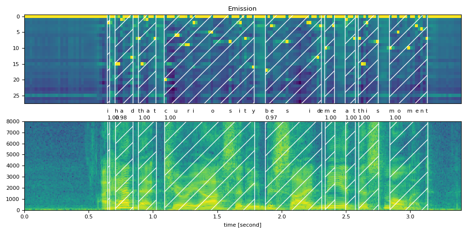
现在让我们看看对齐结果并分割原始将语音转化为文字。

def plot_alignments(waveform, token_spans, emission, transcript, sample_rate=bundle.sample_rate):
    ratio = waveform.size(1) / emission.size(1) / sample_rate

    fig, axes = plt.subplots(2, 1)
    axes[0].imshow(emission[0].detach().cpu().T, aspect="auto")
    axes[0].set_title("Emission")
    axes[0].set_xticks([])

    axes[1].specgram(waveform[0], Fs=sample_rate)
    for t_spans, chars in zip(token_spans, transcript):
        t0, t1 = t_spans[0].start + 0.1, t_spans[-1].end - 0.1
        axes[0].axvspan(t0 - 0.5, t1 - 0.5, facecolor="None", hatch="/", edgecolor="white")
        axes[1].axvspan(ratio * t0, ratio * t1, facecolor="None", hatch="/", edgecolor="white")
        axes[1].annotate(f"{_score(t_spans):.2f}", (ratio * t0, sample_rate * 0.51), annotation_clip=False)

        for span, char in zip(t_spans, chars):
            t0 = span.start * ratio
            axes[1].annotate(char, (t0, sample_rate * 0.55), annotation_clip=False)

    axes[1].set_xlabel("time [second]")
    axes[1].set_xlim([0, None])
    fig.tight_layout()

plot_alignments(waveform, word_spans, emission, TRANSCRIPT)

标记的处理不一致`blank`¶

将令牌级对齐拆分为单词时，您将请注意，某些空白标记的处理方式不同，这使得对结果的解释 somehwat 模棱两可。

当我们绘制分数时，这很容易看出。下图显示单词区域和非单词区域，以及帧级分数的非空令牌。

def plot_scores(word_spans, scores):
    fig, ax = plt.subplots()
    span_xs, span_hs = [], []
    ax.axvspan(word_spans[0][0].start - 0.05, word_spans[-1][-1].end + 0.05, facecolor="paleturquoise", edgecolor="none", zorder=-1)
    for t_span in word_spans:
        for span in t_span:
            for t in range(span.start, span.end):
                span_xs.append(t + 0.5)
                span_hs.append(scores[t].item())
            ax.annotate(LABELS[span.token], (span.start, -0.07))
        ax.axvspan(t_span[0].start - 0.05, t_span[-1].end + 0.05, facecolor="mistyrose", edgecolor="none", zorder=-1)
    ax.bar(span_xs, span_hs, color="lightsalmon", edgecolor="coral")
    ax.set_title("Frame-level scores and word segments")
    ax.set_ylim(-0.1, None)
    ax.grid(True, axis="y")
    ax.axhline(0, color="black")
    fig.tight_layout()


plot_scores(word_spans, alignment_scores)

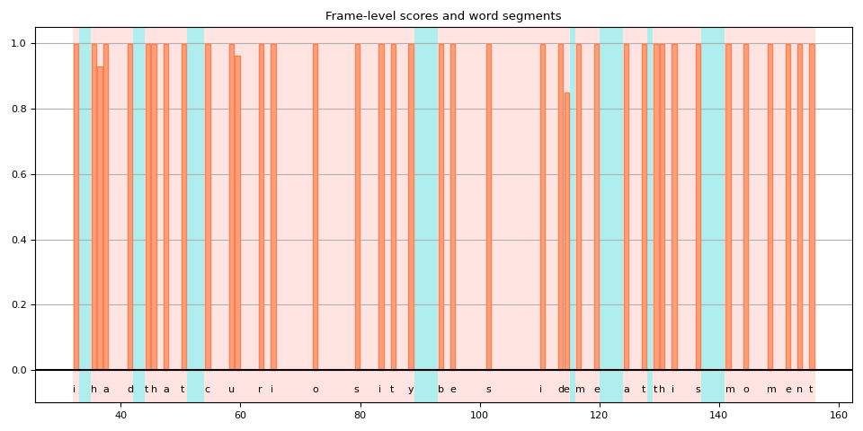
在此图中，空白标记是那些没有竖线。您可以看到，有一些空标记被解释为单词的一部分（突出显示的红色），而其他部分（突出显示的蓝色）不是。

其中一个原因是，该模型是在没有 label 来描述单词 boundary。不仅会处理空白令牌作为重复，但也作为词之间的沉默。

但随之而来的是。应紧接在或在单词的末尾附近 be silent or repeat？

在上面的例子中，如果你回到上一个频谱图和词域，您会看到 “curiosity” 中 “y” 之后，多个 frequency bucket 中仍有一些 activity。

如果这个词中包含那个框架会更准确吗？

不幸的是，CTC 并没有为此提供全面的解决方案。已知使用 CTC 训练的模型表现出“峰值”反应，也就是说，它们往往会因标签的出现而激增，但 spike 不会在标签的持续时间内持续。（注意：预先训练的 Wav2Vec2 模型往往在标签出现次数，但情况并非总是如此。

[Zeyer et al.， 2021] 对 CTC 的。我们鼓励有兴趣了解更多的人参考到报纸。以下是该论文的引述，正是我们面向此处。

在某些情况下，peaky 行为可能会出现问题，例如，当应用程序需要不使用空白标签时，例如，为了获得音素与转录的有意义的时间精确对齐。

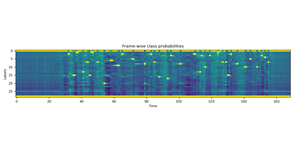
高级：使用令牌处理转录`<star>`¶

现在让我们看看当成绩单部分丢失时，我们该如何使用能够建模的 Token 提高对齐质量 any 令牌。<star>

这里我们使用与上面相同的英文示例。但是我们删除了脚本的 beginning 文本。将音频与此类转录文本对齐会导致现有单词 “this”。但是，可以通过使用标记对缺失的文本进行建模来缓解此问题。“i had that curiosity beside me at”<star>

首先，我们扩展字典以包含标记。<star>

DICTIONARY["*"] = len(DICTIONARY)

接下来，我们使用额外的维度扩展发射张量对应于 token。<star>

star_dim = torch.zeros((1, emission.size(1), 1), device=emission.device, dtype=emission.dtype)
emission = torch.cat((emission, star_dim), 2)

assert len(DICTIONARY) == emission.shape[2]

plot_emission(emission[0])

以下函数组合了所有进程，并计算一次性从 Emission 获得词段。

def compute_alignments(emission, transcript, dictionary):
    tokens = [dictionary[char] for word in transcript for char in word]
    alignment, scores = align(emission, tokens)
    token_spans = F.merge_tokens(alignment, scores)
    word_spans = unflatten(token_spans, [len(word) for word in transcript])
    return word_spans

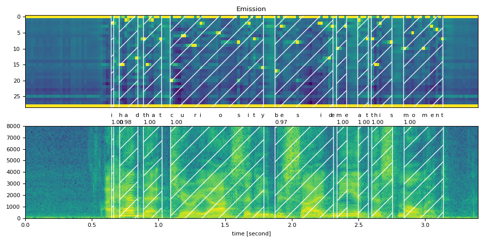
完整文字记录¶

word_spans = compute_alignments(emission, TRANSCRIPT, DICTIONARY)
plot_alignments(waveform, word_spans, emission, TRANSCRIPT)

带标记的部分转录`<star>`¶

现在，我们将 transcript 的第一部分替换为 token。<star>

transcript = "* this moment".split()
word_spans = compute_alignments(emission, transcript, DICTIONARY)
plot_alignments(waveform, word_spans, emission, transcript)

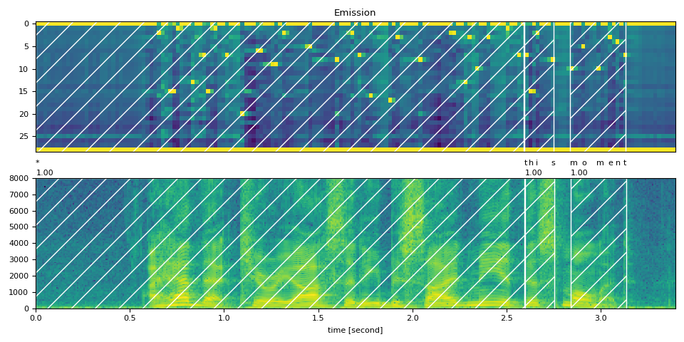
preview_word(waveform, word_spans[0], num_frames, transcript[0])

* (1.00): 0.000 - 2.595 sec

preview_word(waveform, word_spans[1], num_frames, transcript[1])

this (1.00): 2.595 - 2.756 sec

preview_word(waveform, word_spans[2], num_frames, transcript[2])

moment (1.00): 2.837 - 3.138 sec

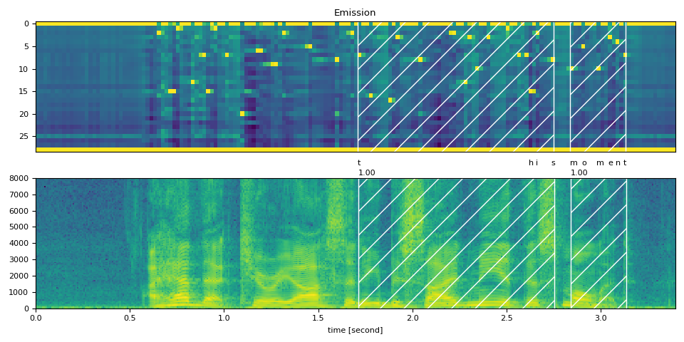
不带标记的部分转录`<star>`¶

作为比较，以下内容对齐了部分转录不使用 Token。它演示了 token 在处理删除错误方面的效果。<star><star>

transcript = "this moment".split()
word_spans = compute_alignments(emission, transcript, DICTIONARY)
plot_alignments(waveform, word_spans, emission, transcript)

结论¶

在本教程中，我们了解了如何使用 torchaudio 的强制对齐用于对齐和分割语音文件的 API，并演示了一种高级用法：在以下情况下，引入 Token 如何提高对齐精度存在转录错误。<star>

确认¶

感谢 Vineel Pratap 和 Zhaoheng Ni 用于开发和开源强制对准器 API。

脚本总运行时间：（0 分 6.927 秒）

由 Sphinx-Gallery 生成的图库

CTC 强制对齐 API 教程¶

制备¶

产生排放¶

标记转录文本¶

计算对标¶

帧级对齐¶

令牌级对齐¶

单词级对齐¶

音频预览¶

可视化¶

标记的处理不一致`blank`¶

高级：使用令牌处理转录`<star>`¶

完整文字记录¶

带标记的部分转录`<star>`¶

不带标记的部分转录`<star>`¶

结论¶

确认¶

文档

教程

资源

CTC 强制对齐 API 教程¶

制备¶

产生排放¶

标记转录文本¶

计算对标¶

帧级对齐¶

令牌级对齐¶

单词级对齐¶

音频预览¶

可视化¶

标记的处理不一致blank¶

高级：使用令牌处理转录<star>¶

完整文字记录¶

带标记的部分转录<star>¶

不带标记的部分转录<star>¶

结论¶

确认¶

文档

教程

资源

标记的处理不一致`blank`¶

高级：使用令牌处理转录`<star>`¶

带标记的部分转录`<star>`¶

不带标记的部分转录`<star>`¶