注意
点击 这里 下载完整示例代码
滤波器设计教程
作者: Moto Hira
本教程展示了如何创建基本的数字滤波器(脉冲响应)及其特性。
我们研究基于窗口化sinc核以及频率采样方法的低通、高通和带通滤波器。
import torch
import torchaudio

print(torch.__version__)
print(torchaudio.__version__)

import matplotlib.pyplot as plt
2.4.0
2.4.0
from torchaudio.prototype.functional import frequency_impulse_response, sinc_impulse_response
窗函数-Sinc滤波器
正弦滤波器 是一种 理想化的滤波器,它可以去除高于截止频率的频率, 而不影响较低频率。
Sinc滤波器在解析解中具有无限的滤波宽度。 在数值计算中,sinc滤波器无法精确表达, 因此需要进行近似处理。
窗函数sinc有限脉冲响应是sinc滤波器的一种近似。它是通过首先对给定的截止频率计算sinc函数,然后截断滤波器裙部,并应用如汉明窗等窗函数以减少截断引入的伪影来获得的。
sinc_impulse_response()
生成给定截止频率的窗函数sinc脉冲响应。
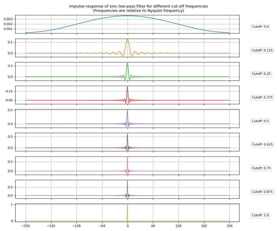
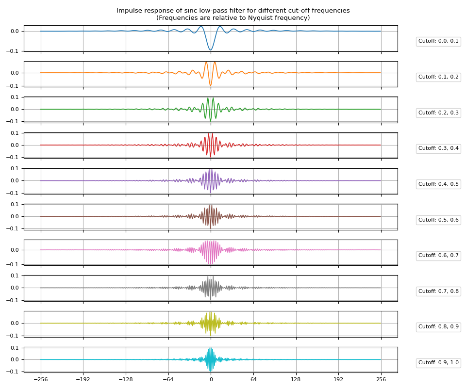
低通滤波器
脉冲响应
创建sinc IR就像将截止频率值传递给
sinc_impulse_response()。
Cutoff shape: torch.Size([9])
Impulse response shape: torch.Size([9, 513])
让我们可视化得到的脉冲响应。
def plot_sinc_ir(irs, cutoff):
    num_filts, window_size = irs.shape
    half = window_size // 2

    fig, axes = plt.subplots(num_filts, 1, sharex=True, figsize=(9.6, 8))
    t = torch.linspace(-half, half - 1, window_size)
    for ax, ir, coff, color in zip(axes, irs, cutoff, plt.cm.tab10.colors):
        ax.plot(t, ir, linewidth=1.2, color=color, zorder=4, label=f"Cutoff: {coff}")
        ax.legend(loc=(1.05, 0.2), handletextpad=0, handlelength=0)
        ax.grid(True)
    fig.suptitle(
        "Impulse response of sinc low-pass filter for different cut-off frequencies\n"
        "(Frequencies are relative to Nyquist frequency)"
    )
    axes[-1].set_xticks([i * half // 4 for i in range(-4, 5)])
    fig.tight_layout()
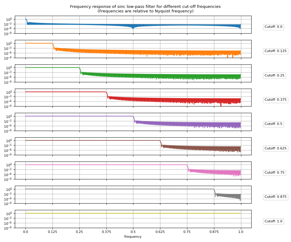
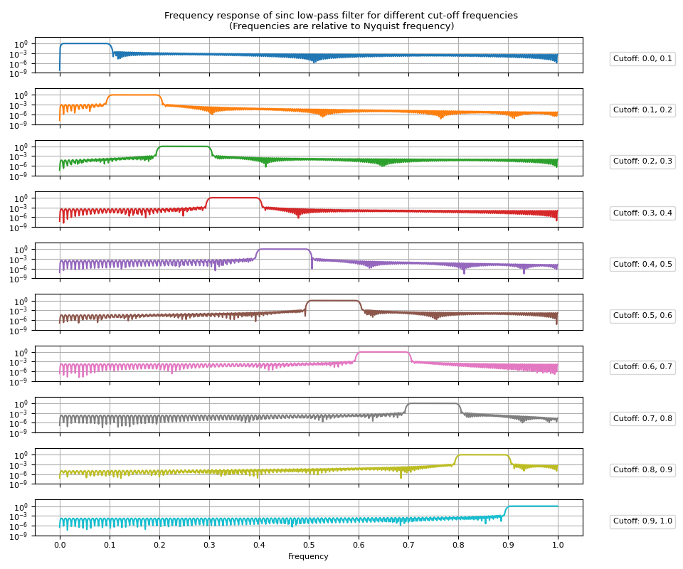
频率响应
接下来,让我们看一下频率响应。 简单地对脉冲响应应用傅里叶变换就可以得到频率响应。
frs = torch.fft.rfft(irs, n=2048, dim=1).abs()
让我们可视化得到的频率响应。
def plot_sinc_fr(frs, cutoff, band=False):
    num_filts, num_fft = frs.shape
    num_ticks = num_filts + 1 if band else num_filts

    fig, axes = plt.subplots(num_filts, 1, sharex=True, sharey=True, figsize=(9.6, 8))
    for ax, fr, coff, color in zip(axes, frs, cutoff, plt.cm.tab10.colors):
        ax.grid(True)
        ax.semilogy(fr, color=color, zorder=4, label=f"Cutoff: {coff}")
        ax.legend(loc=(1.05, 0.2), handletextpad=0, handlelength=0).set_zorder(3)
    axes[-1].set(
        ylim=[None, 100],
        yticks=[1e-9, 1e-6, 1e-3, 1],
        xticks=torch.linspace(0, num_fft, num_ticks),
        xticklabels=[f"{i/(num_ticks - 1)}" for i in range(num_ticks)],
        xlabel="Frequency",
    )
    fig.suptitle(
        "Frequency response of sinc low-pass filter for different cut-off frequencies\n"
        "(Frequencies are relative to Nyquist frequency)"
    )
    fig.tight_layout()
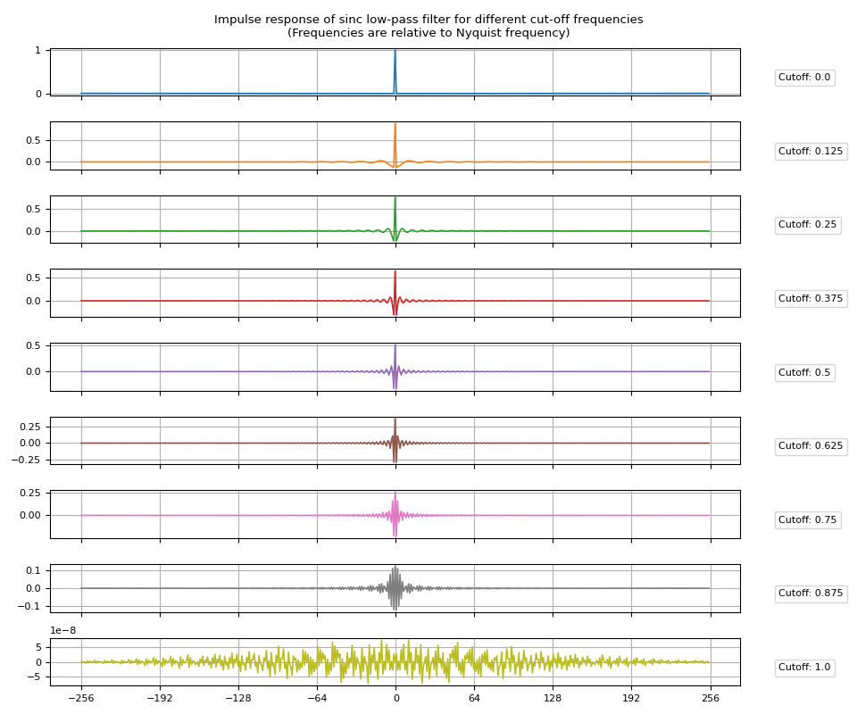
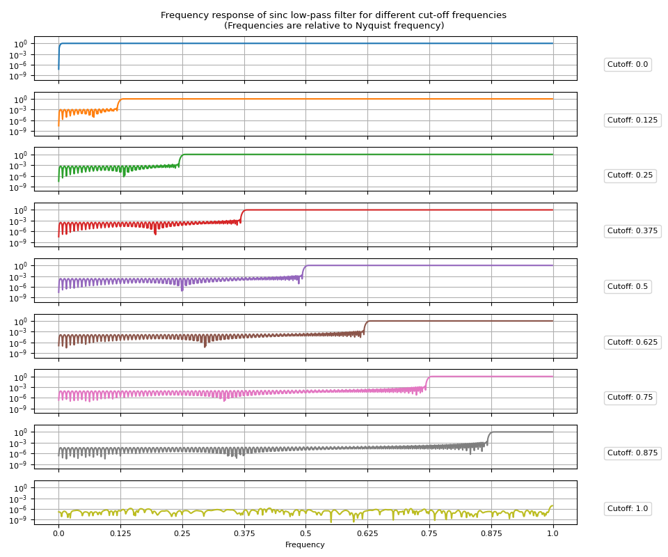
高通滤波器
高通滤波器可以通过从狄拉克δ函数中减去低通脉冲响应来获得。
传递 high_pass=True 到
sinc_impulse_response()
将把返回的滤波器核更改为高通滤波器。
irs = sinc_impulse_response(cutoff, window_size=513, high_pass=True)
frs = torch.fft.rfft(irs, n=2048, dim=1).abs()
脉冲响应
频率响应
带通滤波器
带通滤波器可以通过从低频带的低通滤波器中减去高频带的低通滤波器来获得。
脉冲响应
频率响应
频率采样
我们接下来要研究的方法从期望的频率响应开始,通过应用逆傅里叶变换来获得脉冲响应。
frequency_impulse_response()
采用(未归一化)频率的幅度分布,并
从中构造脉冲响应。
然而需要注意的是,得到的脉冲响应并不能产生所需的频率响应。
在下面的内容中,我们将创建多个滤波器,并比较输入的频率响应和实际的频率响应。
砖墙滤波器
让我们从砖墙滤波器开始
magnitudes = torch.concat([torch.ones((128,)), torch.zeros((128,))])
ir = frequency_impulse_response(magnitudes)

print("Magnitudes:", magnitudes.shape)
print("Impulse Response:", ir.shape)
Magnitudes: torch.Size([256])
Impulse Response: torch.Size([510])
def plot_ir(magnitudes, ir, num_fft=2048):
    fr = torch.fft.rfft(ir, n=num_fft, dim=0).abs()
    ir_size = ir.size(-1)
    half = ir_size // 2

    fig, axes = plt.subplots(3, 1)
    t = torch.linspace(-half, half - 1, ir_size)
    axes[0].plot(t, ir)
    axes[0].grid(True)
    axes[0].set(title="Impulse Response")
    axes[0].set_xticks([i * half // 4 for i in range(-4, 5)])
    t = torch.linspace(0, 1, fr.numel())
    axes[1].plot(t, fr, label="Actual")
    axes[2].semilogy(t, fr, label="Actual")
    t = torch.linspace(0, 1, magnitudes.numel())
    for i in range(1, 3):
        axes[i].plot(t, magnitudes, label="Desired (input)", linewidth=1.1, linestyle="--")
        axes[i].grid(True)
    axes[1].set(title="Frequency Response")
    axes[2].set(title="Frequency Response (log-scale)", xlabel="Frequency")
    axes[2].legend(loc="center right")
    fig.tight_layout()
plot_ir(magnitudes, ir)
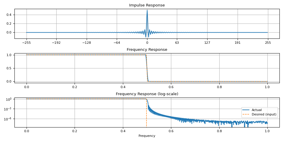
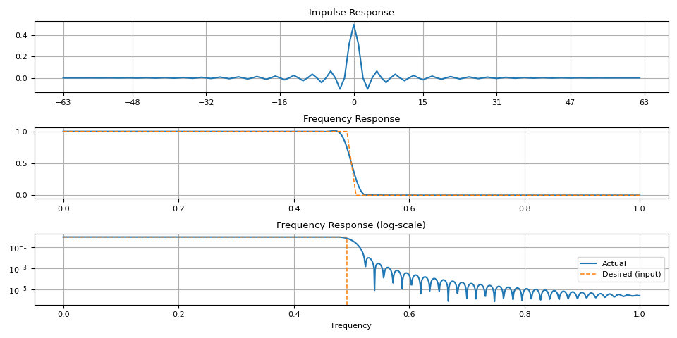
请注意过渡带周围存在一些伪影。当窗口尺寸较小时,这种现象会更加明显。
magnitudes = torch.concat([torch.ones((32,)), torch.zeros((32,))])
ir = frequency_impulse_response(magnitudes)
plot_ir(magnitudes, ir)
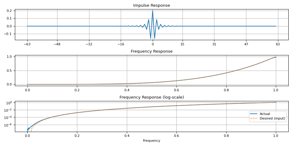
任意形状
magnitudes = torch.linspace(0, 1, 64) ** 4.0
ir = frequency_impulse_response(magnitudes)
plot_ir(magnitudes, ir)
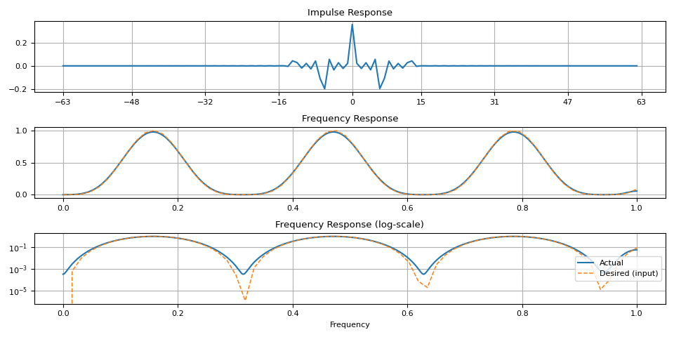
magnitudes = torch.sin(torch.linspace(0, 10, 64)) ** 4.0
ir = frequency_impulse_response(magnitudes)
plot_ir(magnitudes, ir)
参考文献
https://www.analog.com/media/en/technical-documentation/dsp-book/dsp_book_Ch16.pdf
https://courses.engr.illinois.edu/ece401/fa2020/slides/lec10.pdf
https://ccrma.stanford.edu/~jos/sasp/Windowing_Desired_Impulse_Response.html
脚本的总运行时间: ( 0 分钟 5.351 秒)