注意
点击 这里 下载完整示例代码
CTC 强制对齐 API 教程
强制对齐是一个将文本转录与语音对齐的过程。
本教程展示了如何使用
torchaudio.functional.forced_align() 将文本转录与语音对齐,该工具是随着
将语音技术扩展到1,000多种语言 的工作一起开发的。
forced_align() 提供了自定义的 CPU 和 CUDA 实现,其性能优于上面的纯 Python 实现,并且更加准确。
它还可以通过特殊的 <star> 令牌处理缺失的转录文本。
此外还有一个高级API,torchaudio.pipelines.Wav2Vec2FABundle,
它封装了本教程中讲解的预处理和后处理步骤,使强制对齐的运行更加简便。
多语言数据的强制对齐使用此API来
说明如何对非英语字幕进行对齐。
准备
import torch
import torchaudio

print(torch.__version__)
print(torchaudio.__version__)
2.4.0
2.4.0
device = torch.device("cuda" if torch.cuda.is_available() else "cpu")
print(device)
cuda
import IPython
import matplotlib.pyplot as plt

import torchaudio.functional as F
首先我们准备要使用的语音数据和转录文本。
SPEECH_FILE = torchaudio.utils.download_asset("tutorial-assets/Lab41-SRI-VOiCES-src-sp0307-ch127535-sg0042.wav")
waveform, _ = torchaudio.load(SPEECH_FILE)
TRANSCRIPT = "i had that curiosity beside me at this moment".split()
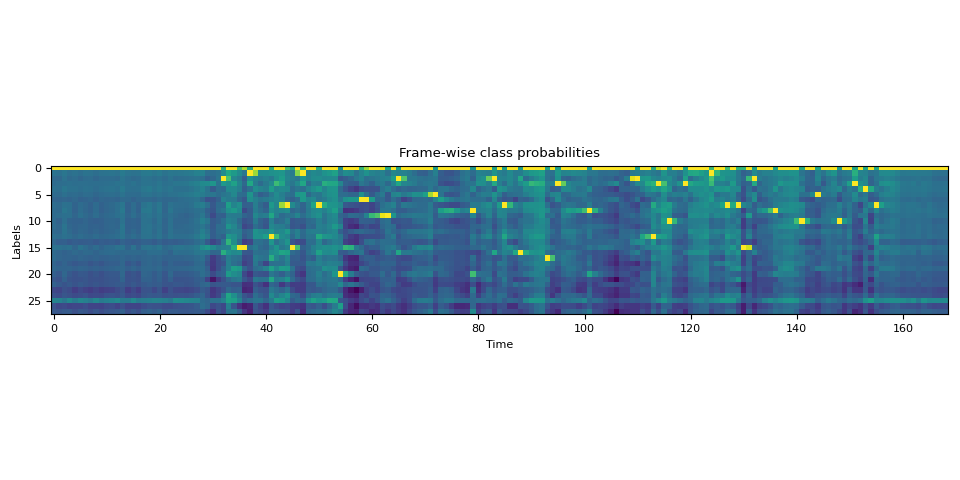
生成排放量
forced_align() 接收发射和
token 序列,并输出 token 的时间戳及其得分。
发射表示的是对 token 的逐帧概率分布,可以通过将波形传递给声学模型来获得。
词元是文本的数值表达形式。对文本进行词元化的方法有很多种,但在这里,我们简单地将字母映射为整数,这与我们将要使用的声学模型在训练时构建标签的方式一致。
我们将使用一个预训练的Wav2Vec2模型,
torchaudio.pipelines.MMS_FA,来获取发射并标记
转录文本。
bundle = torchaudio.pipelines.MMS_FA

model = bundle.get_model(with_star=False).to(device)
with torch.inference_mode():
    emission, _ = model(waveform.to(device))
Downloading: "https://dl.fbaipublicfiles.com/mms/torchaudio/ctc_alignment_mling_uroman/model.pt" to /root/.cache/torch/hub/checkpoints/model.pt

  0%|          | 0.00/1.18G [00:00<?, ?B/s]
  0%|          | 128k/1.18G [00:00<26:01, 808kB/s]
  0%|          | 384k/1.18G [00:00<15:06, 1.39MB/s]
  0%|          | 640k/1.18G [00:00<12:36, 1.67MB/s]
  0%|          | 1.00M/1.18G [00:00<09:15, 2.27MB/s]
  0%|          | 1.25M/1.18G [00:00<09:25, 2.23MB/s]
  0%|          | 1.62M/1.18G [00:00<08:12, 2.56MB/s]
  0%|          | 2.00M/1.18G [00:00<07:33, 2.78MB/s]
  0%|          | 2.38M/1.18G [00:01<07:10, 2.93MB/s]
  0%|          | 2.88M/1.18G [00:01<06:17, 3.34MB/s]
  0%|          | 3.38M/1.18G [00:01<05:44, 3.66MB/s]
  0%|          | 3.88M/1.18G [00:01<05:14, 4.00MB/s]
  0%|          | 4.38M/1.18G [00:01<05:05, 4.11MB/s]
  0%|          | 4.88M/1.18G [00:01<05:00, 4.18MB/s]
  0%|          | 5.62M/1.18G [00:01<04:17, 4.89MB/s]
  1%|          | 6.38M/1.18G [00:01<04:02, 5.18MB/s]
  1%|          | 7.25M/1.18G [00:02<03:47, 5.51MB/s]
  1%|          | 8.25M/1.18G [00:02<03:16, 6.38MB/s]
  1%|          | 9.25M/1.18G [00:02<02:57, 7.05MB/s]
  1%|          | 10.5M/1.18G [00:02<02:33, 8.13MB/s]
  1%|          | 11.8M/1.18G [00:02<02:20, 8.91MB/s]
  1%|1         | 13.1M/1.18G [00:02<02:07, 9.79MB/s]
  1%|1         | 14.8M/1.18G [00:02<01:52, 11.0MB/s]
  1%|1         | 16.5M/1.18G [00:02<01:41, 12.2MB/s]
  2%|1         | 18.4M/1.18G [00:03<01:32, 13.4MB/s]
  2%|1         | 20.5M/1.18G [00:03<01:23, 14.8MB/s]
  2%|1         | 22.8M/1.18G [00:03<01:16, 16.2MB/s]
  2%|2         | 25.2M/1.18G [00:03<01:09, 17.8MB/s]
  2%|2         | 28.1M/1.18G [00:03<01:02, 19.8MB/s]
  3%|2         | 30.1M/1.18G [00:03<01:01, 19.9MB/s]
  3%|2         | 32.9M/1.18G [00:03<00:57, 21.3MB/s]
  3%|3         | 36.4M/1.18G [00:03<00:50, 24.0MB/s]
  3%|3         | 40.4M/1.18G [00:03<00:44, 27.2MB/s]
  4%|3         | 44.8M/1.18G [00:04<00:40, 30.3MB/s]
  4%|4         | 49.5M/1.18G [00:04<00:36, 33.6MB/s]
  5%|4         | 54.8M/1.18G [00:04<00:32, 37.2MB/s]
  5%|5         | 60.6M/1.18G [00:04<00:29, 41.0MB/s]
  6%|5         | 66.4M/1.18G [00:04<00:27, 43.5MB/s]
  6%|6         | 73.4M/1.18G [00:04<00:24, 48.6MB/s]
  7%|6         | 81.0M/1.18G [00:04<00:22, 52.3MB/s]
  7%|7         | 88.0M/1.18G [00:05<00:26, 43.6MB/s]
  8%|7         | 94.4M/1.18G [00:05<00:30, 38.6MB/s]
  8%|8         | 98.4M/1.18G [00:05<00:30, 38.0MB/s]
  9%|8         | 103M/1.18G [00:05<00:28, 40.5MB/s]
  9%|9         | 110M/1.18G [00:05<00:26, 43.6MB/s]
 10%|9         | 116M/1.18G [00:05<00:25, 44.4MB/s]
 10%|9         | 120M/1.18G [00:06<00:40, 28.4MB/s]
 11%|#         | 127M/1.18G [00:06<00:31, 35.5MB/s]
 11%|#1        | 135M/1.18G [00:06<00:27, 41.4MB/s]
 12%|#1        | 142M/1.18G [00:06<00:25, 43.9MB/s]
 12%|#2        | 149M/1.18G [00:06<00:22, 48.6MB/s]
 13%|#2        | 156M/1.18G [00:06<00:22, 47.8MB/s]
 14%|#3        | 163M/1.18G [00:06<00:21, 51.8MB/s]
 14%|#4        | 169M/1.18G [00:07<00:25, 41.8MB/s]
 14%|#4        | 174M/1.18G [00:07<00:23, 45.5MB/s]
 15%|#4        | 179M/1.18G [00:07<00:24, 44.5MB/s]
 15%|#5        | 184M/1.18G [00:07<00:24, 43.5MB/s]
 16%|#5        | 190M/1.18G [00:07<00:27, 39.2MB/s]
 16%|#6        | 194M/1.18G [00:07<00:29, 35.6MB/s]
 16%|#6        | 198M/1.18G [00:07<00:28, 36.8MB/s]
 17%|#6        | 202M/1.18G [00:08<00:30, 34.0MB/s]
 17%|#7        | 206M/1.18G [00:08<00:36, 28.8MB/s]
 18%|#7        | 212M/1.18G [00:08<00:31, 32.6MB/s]
 18%|#8        | 218M/1.18G [00:08<00:27, 38.1MB/s]
 19%|#8        | 223M/1.18G [00:08<00:25, 40.8MB/s]
 19%|#8        | 228M/1.18G [00:08<00:24, 42.3MB/s]
 19%|#9        | 232M/1.18G [00:08<00:24, 40.8MB/s]
 20%|#9        | 238M/1.18G [00:09<00:26, 38.1MB/s]
 20%|##        | 242M/1.18G [00:09<00:27, 36.2MB/s]
 21%|##        | 247M/1.18G [00:09<00:26, 38.5MB/s]
 21%|##1       | 255M/1.18G [00:09<00:22, 44.9MB/s]
 22%|##1       | 261M/1.18G [00:09<00:20, 49.2MB/s]
 22%|##2       | 266M/1.18G [00:09<00:20, 48.2MB/s]
 22%|##2       | 271M/1.18G [00:09<00:21, 45.1MB/s]
 23%|##2       | 276M/1.18G [00:09<00:22, 43.2MB/s]
 23%|##3       | 280M/1.18G [00:10<00:34, 28.0MB/s]
 24%|##3       | 286M/1.18G [00:10<00:27, 34.9MB/s]
 24%|##4       | 291M/1.18G [00:10<00:29, 32.7MB/s]
 25%|##4       | 295M/1.18G [00:10<00:27, 35.0MB/s]
 25%|##4       | 300M/1.18G [00:10<00:26, 36.0MB/s]
 25%|##5       | 304M/1.18G [00:10<00:28, 33.3MB/s]
 26%|##5       | 311M/1.18G [00:11<00:21, 42.8MB/s]
 26%|##6       | 316M/1.18G [00:11<00:24, 38.5MB/s]
 27%|##6       | 320M/1.18G [00:11<00:28, 32.1MB/s]
 27%|##7       | 328M/1.18G [00:11<00:23, 39.6MB/s]
 28%|##7       | 332M/1.18G [00:11<00:23, 38.3MB/s]
 28%|##7       | 336M/1.18G [00:11<00:27, 32.7MB/s]
 28%|##8       | 340M/1.18G [00:11<00:28, 31.8MB/s]
 29%|##8       | 344M/1.18G [00:12<00:27, 33.0MB/s]
 29%|##8       | 347M/1.18G [00:12<00:29, 30.0MB/s]
 29%|##9       | 354M/1.18G [00:12<00:24, 35.9MB/s]
 30%|##9       | 358M/1.18G [00:12<00:23, 37.1MB/s]
 30%|###       | 362M/1.18G [00:12<00:30, 29.1MB/s]
 31%|###       | 368M/1.18G [00:12<00:25, 34.1MB/s]
 31%|###       | 372M/1.18G [00:12<00:25, 34.3MB/s]
 31%|###1      | 376M/1.18G [00:13<00:25, 34.1MB/s]
 32%|###1      | 382M/1.18G [00:13<00:21, 40.1MB/s]
 32%|###2      | 386M/1.18G [00:13<00:22, 38.9MB/s]
 32%|###2      | 390M/1.18G [00:13<00:22, 37.9MB/s]
 33%|###3      | 397M/1.18G [00:13<00:18, 46.5MB/s]
 33%|###3      | 403M/1.18G [00:13<00:17, 48.2MB/s]
 34%|###4      | 411M/1.18G [00:13<00:14, 56.3MB/s]
 35%|###4      | 416M/1.18G [00:13<00:14, 56.4MB/s]
 35%|###5      | 422M/1.18G [00:13<00:14, 55.5MB/s]
 36%|###5      | 428M/1.18G [00:14<00:15, 52.1MB/s]
 36%|###6      | 434M/1.18G [00:14<00:16, 48.8MB/s]
 37%|###6      | 440M/1.18G [00:14<00:18, 42.8MB/s]
 37%|###7      | 448M/1.18G [00:14<00:16, 48.0MB/s]
 38%|###7      | 452M/1.18G [00:14<00:16, 48.5MB/s]
 38%|###8      | 459M/1.18G [00:14<00:16, 48.6MB/s]
 39%|###8      | 466M/1.18G [00:14<00:14, 52.1MB/s]
 39%|###9      | 474M/1.18G [00:15<00:13, 55.1MB/s]
 40%|###9      | 480M/1.18G [00:15<00:15, 49.9MB/s]
 41%|####      | 488M/1.18G [00:15<00:14, 51.9MB/s]
 41%|####      | 493M/1.18G [00:15<00:15, 48.3MB/s]
 41%|####1     | 497M/1.18G [00:15<00:18, 39.7MB/s]
 42%|####1     | 504M/1.18G [00:15<00:17, 43.0MB/s]
 42%|####2     | 508M/1.18G [00:15<00:18, 40.0MB/s]
 43%|####2     | 512M/1.18G [00:16<00:21, 33.4MB/s]
 43%|####3     | 518M/1.18G [00:16<00:18, 39.5MB/s]
 43%|####3     | 523M/1.18G [00:16<00:17, 41.5MB/s]
 44%|####3     | 527M/1.18G [00:16<00:16, 42.0MB/s]
 44%|####4     | 531M/1.18G [00:16<00:17, 40.9MB/s]
 44%|####4     | 536M/1.18G [00:16<00:17, 39.7MB/s]
 45%|####4     | 540M/1.18G [00:16<00:18, 38.0MB/s]
 45%|####5     | 546M/1.18G [00:16<00:15, 43.2MB/s]
 46%|####5     | 553M/1.18G [00:17<00:13, 50.2MB/s]
 46%|####6     | 558M/1.18G [00:17<00:13, 48.6MB/s]
 47%|####6     | 564M/1.18G [00:17<00:14, 45.1MB/s]
 47%|####7     | 568M/1.18G [00:17<00:16, 40.9MB/s]
 48%|####7     | 574M/1.18G [00:17<00:15, 42.6MB/s]
 48%|####8     | 579M/1.18G [00:17<00:16, 39.8MB/s]
 48%|####8     | 583M/1.18G [00:17<00:15, 40.8MB/s]
 49%|####8     | 587M/1.18G [00:17<00:16, 39.7MB/s]
 49%|####9     | 591M/1.18G [00:18<00:16, 38.9MB/s]
 49%|####9     | 595M/1.18G [00:18<00:18, 35.4MB/s]
 50%|####9     | 600M/1.18G [00:18<00:17, 37.2MB/s]
 50%|#####     | 604M/1.18G [00:18<00:16, 37.8MB/s]
 51%|#####     | 611M/1.18G [00:18<00:12, 48.0MB/s]
 51%|#####1    | 616M/1.18G [00:18<00:13, 46.4MB/s]
 52%|#####1    | 622M/1.18G [00:18<00:12, 48.0MB/s]
 52%|#####2    | 628M/1.18G [00:18<00:12, 49.7MB/s]
 53%|#####2    | 635M/1.18G [00:19<00:11, 53.5MB/s]
 53%|#####3    | 643M/1.18G [00:19<00:10, 56.2MB/s]
 54%|#####4    | 650M/1.18G [00:19<00:10, 57.9MB/s]
 55%|#####4    | 657M/1.18G [00:19<00:09, 61.6MB/s]
 55%|#####5    | 664M/1.18G [00:19<00:09, 59.0MB/s]
 56%|#####5    | 670M/1.18G [00:19<00:09, 60.0MB/s]
 56%|#####6    | 677M/1.18G [00:19<00:09, 60.7MB/s]
 57%|#####6    | 684M/1.18G [00:19<00:08, 61.3MB/s]
 57%|#####7    | 691M/1.18G [00:19<00:08, 63.1MB/s]
 58%|#####7    | 697M/1.18G [00:20<00:09, 54.1MB/s]
 58%|#####8    | 702M/1.18G [00:20<00:09, 53.1MB/s]
 59%|#####8    | 708M/1.18G [00:20<00:11, 47.2MB/s]
 59%|#####9    | 712M/1.18G [00:20<00:12, 40.3MB/s]
 60%|#####9    | 720M/1.18G [00:20<00:11, 45.1MB/s]
 60%|######    | 724M/1.18G [00:20<00:12, 41.4MB/s]
 60%|######    | 728M/1.18G [00:21<00:15, 32.8MB/s]
 61%|######1   | 736M/1.18G [00:21<00:12, 39.5MB/s]
 61%|######1   | 740M/1.18G [00:21<00:12, 37.5MB/s]
 62%|######1   | 744M/1.18G [00:21<00:12, 38.2MB/s]
 62%|######2   | 751M/1.18G [00:21<00:10, 44.9MB/s]
 63%|######3   | 758M/1.18G [00:21<00:09, 51.5MB/s]
 63%|######3   | 764M/1.18G [00:21<00:09, 46.9MB/s]
 64%|######4   | 771M/1.18G [00:21<00:09, 49.7MB/s]
 64%|######4   | 776M/1.18G [00:22<00:10, 44.7MB/s]
 65%|######5   | 784M/1.18G [00:22<00:08, 49.0MB/s]
 66%|######5   | 789M/1.18G [00:22<00:08, 51.1MB/s]
 66%|######5   | 794M/1.18G [00:22<00:08, 50.7MB/s]
 66%|######6   | 799M/1.18G [00:22<00:08, 49.2MB/s]
 67%|######6   | 806M/1.18G [00:22<00:08, 51.4MB/s]
 67%|######7   | 812M/1.18G [00:22<00:08, 47.7MB/s]
 68%|######8   | 818M/1.18G [00:22<00:08, 50.0MB/s]
 68%|######8   | 824M/1.18G [00:23<00:08, 46.5MB/s]
 69%|######8   | 830M/1.18G [00:23<00:09, 43.1MB/s]
 69%|######9   | 835M/1.18G [00:23<00:09, 42.3MB/s]
 70%|######9   | 839M/1.18G [00:23<00:10, 35.9MB/s]
 70%|######9   | 842M/1.18G [00:23<00:10, 36.1MB/s]
 70%|#######   | 848M/1.18G [00:23<00:09, 38.7MB/s]
 71%|#######   | 852M/1.18G [00:23<00:09, 38.1MB/s]
 71%|#######1  | 858M/1.18G [00:24<00:08, 44.9MB/s]
 72%|#######1  | 864M/1.18G [00:24<00:07, 47.5MB/s]
 72%|#######2  | 871M/1.18G [00:24<00:06, 50.2MB/s]
 73%|#######2  | 876M/1.18G [00:24<00:07, 45.0MB/s]
 73%|#######3  | 883M/1.18G [00:24<00:06, 50.2MB/s]
 74%|#######3  | 890M/1.18G [00:24<00:06, 52.4MB/s]
 74%|#######4  | 897M/1.18G [00:24<00:06, 53.1MB/s]
 75%|#######5  | 904M/1.18G [00:24<00:05, 57.6MB/s]
 76%|#######5  | 910M/1.18G [00:24<00:05, 57.2MB/s]
 76%|#######6  | 916M/1.18G [00:25<00:05, 52.7MB/s]
 77%|#######6  | 921M/1.18G [00:25<00:06, 44.0MB/s]
 77%|#######6  | 926M/1.18G [00:25<00:07, 39.8MB/s]
 77%|#######7  | 930M/1.18G [00:25<00:07, 37.6MB/s]
 78%|#######7  | 934M/1.18G [00:25<00:08, 32.0MB/s]
 78%|#######7  | 938M/1.18G [00:25<00:08, 32.3MB/s]
 78%|#######8  | 944M/1.18G [00:26<00:07, 37.1MB/s]
 79%|#######8  | 948M/1.18G [00:26<00:06, 39.5MB/s]
 79%|#######9  | 954M/1.18G [00:26<00:05, 44.4MB/s]
 80%|#######9  | 960M/1.18G [00:26<00:06, 37.3MB/s]
 80%|########  | 966M/1.18G [00:26<00:06, 40.2MB/s]
 81%|########  | 971M/1.18G [00:26<00:05, 42.9MB/s]
 81%|########1 | 976M/1.18G [00:26<00:05, 41.8MB/s]
 81%|########1 | 980M/1.18G [00:26<00:05, 42.4MB/s]
 82%|########1 | 984M/1.18G [00:27<00:06, 33.9MB/s]
 82%|########2 | 990M/1.18G [00:27<00:05, 38.8MB/s]
 83%|########2 | 994M/1.18G [00:27<00:05, 38.2MB/s]
 83%|########3 | 999M/1.18G [00:27<00:05, 40.2MB/s]
 83%|########3 | 0.98G/1.18G [00:27<00:05, 39.3MB/s]
 84%|########3 | 0.98G/1.18G [00:27<00:05, 38.1MB/s]
 84%|########4 | 0.99G/1.18G [00:27<00:04, 40.9MB/s]
 85%|########4 | 1.00G/1.18G [00:28<00:04, 40.4MB/s]
 85%|########5 | 1.00G/1.18G [00:28<00:04, 42.6MB/s]
 86%|########5 | 1.01G/1.18G [00:28<00:03, 46.9MB/s]
 86%|########6 | 1.01G/1.18G [00:28<00:03, 50.9MB/s]
 87%|########6 | 1.02G/1.18G [00:28<00:03, 51.7MB/s]
 87%|########7 | 1.03G/1.18G [00:28<00:02, 54.6MB/s]
 88%|########8 | 1.04G/1.18G [00:28<00:02, 56.8MB/s]
 89%|########8 | 1.04G/1.18G [00:28<00:02, 48.4MB/s]
 89%|########8 | 1.05G/1.18G [00:29<00:03, 40.7MB/s]
 89%|########9 | 1.05G/1.18G [00:29<00:03, 40.3MB/s]
 90%|########9 | 1.05G/1.18G [00:29<00:03, 39.2MB/s]
 90%|######### | 1.06G/1.18G [00:29<00:02, 44.7MB/s]
 91%|######### | 1.07G/1.18G [00:29<00:02, 44.4MB/s]
 91%|#########1| 1.07G/1.18G [00:29<00:02, 39.9MB/s]
 92%|#########1| 1.08G/1.18G [00:29<00:02, 44.6MB/s]
 92%|#########1| 1.08G/1.18G [00:29<00:02, 44.7MB/s]
 92%|#########2| 1.09G/1.18G [00:30<00:02, 34.3MB/s]
 93%|#########2| 1.09G/1.18G [00:30<00:02, 35.2MB/s]
 93%|#########3| 1.10G/1.18G [00:30<00:02, 41.6MB/s]
 94%|#########3| 1.10G/1.18G [00:30<00:01, 47.5MB/s]
 94%|#########4| 1.11G/1.18G [00:30<00:01, 51.1MB/s]
 95%|#########4| 1.11G/1.18G [00:30<00:01, 49.6MB/s]
 95%|#########5| 1.12G/1.18G [00:30<00:01, 50.3MB/s]
 96%|#########6| 1.13G/1.18G [00:31<00:00, 54.7MB/s]
 96%|#########6| 1.13G/1.18G [00:31<00:00, 52.6MB/s]
 97%|#########7| 1.14G/1.18G [00:31<00:00, 53.7MB/s]
 98%|#########7| 1.15G/1.18G [00:31<00:00, 57.1MB/s]
 98%|#########8| 1.15G/1.18G [00:31<00:00, 43.9MB/s]
 99%|#########8| 1.16G/1.18G [00:31<00:00, 47.5MB/s]
 99%|#########8| 1.16G/1.18G [00:31<00:00, 43.7MB/s]
 99%|#########9| 1.17G/1.18G [00:31<00:00, 43.8MB/s]
100%|#########9| 1.17G/1.18G [00:32<00:00, 42.6MB/s]
100%|##########| 1.18G/1.18G [00:32<00:00, 39.2MB/s]
对转录文本进行分词
我们创建一个字典,将每个标签映射到对应的标记。
LABELS = bundle.get_labels(star=None)
DICTIONARY = bundle.get_dict(star=None)
for k, v in DICTIONARY.items():
    print(f"{k}: {v}")
-: 0
a: 1
i: 2
e: 3
n: 4
o: 5
u: 6
t: 7
s: 8
r: 9
m: 10
k: 11
l: 12
d: 13
g: 14
h: 15
y: 16
b: 17
p: 18
w: 19
c: 20
v: 21
j: 22
z: 23
f: 24
': 25
q: 26
x: 27
将文本转换为标记(tokens)就像
tokenized_transcript = [DICTIONARY[c] for word in TRANSCRIPT for c in word]

for t in tokenized_transcript:
    print(t, end=" ")
print()
2 15 1 13 7 15 1 7 20 6 9 2 5 8 2 7 16 17 3 8 2 13 3 10 3 1 7 7 15 2 8 10 5 10 3 4 7
计算对齐
帧级对齐
现在我们调用TorchAudio的强制对齐API来计算
帧级别的对齐。如需了解函数签名的详细信息,请参阅 forced_align()。
def align(emission, tokens):
    targets = torch.tensor([tokens], dtype=torch.int32, device=device)
    alignments, scores = F.forced_align(emission, targets, blank=0)

    alignments, scores = alignments[0], scores[0]  # remove batch dimension for simplicity
    scores = scores.exp()  # convert back to probability
    return alignments, scores


aligned_tokens, alignment_scores = align(emission, tokenized_transcript)
现在让我们看一下输出。
for i, (ali, score) in enumerate(zip(aligned_tokens, alignment_scores)):
    print(f"{i:3d}:\t{ali:2d} [{LABELS[ali]}], {score:.2f}")
  0:     0 [-], 1.00
  1:     0 [-], 1.00
  2:     0 [-], 1.00
  3:     0 [-], 1.00
  4:     0 [-], 1.00
  5:     0 [-], 1.00
  6:     0 [-], 1.00
  7:     0 [-], 1.00
  8:     0 [-], 1.00
  9:     0 [-], 1.00
 10:     0 [-], 1.00
 11:     0 [-], 1.00
 12:     0 [-], 1.00
 13:     0 [-], 1.00
 14:     0 [-], 1.00
 15:     0 [-], 1.00
 16:     0 [-], 1.00
 17:     0 [-], 1.00
 18:     0 [-], 1.00
 19:     0 [-], 1.00
 20:     0 [-], 1.00
 21:     0 [-], 1.00
 22:     0 [-], 1.00
 23:     0 [-], 1.00
 24:     0 [-], 1.00
 25:     0 [-], 1.00
 26:     0 [-], 1.00
 27:     0 [-], 1.00
 28:     0 [-], 1.00
 29:     0 [-], 1.00
 30:     0 [-], 1.00
 31:     0 [-], 1.00
 32:     2 [i], 1.00
 33:     0 [-], 1.00
 34:     0 [-], 1.00
 35:    15 [h], 1.00
 36:    15 [h], 0.93
 37:     1 [a], 1.00
 38:     0 [-], 0.96
 39:     0 [-], 1.00
 40:     0 [-], 1.00
 41:    13 [d], 1.00
 42:     0 [-], 1.00
 43:     0 [-], 0.97
 44:     7 [t], 1.00
 45:    15 [h], 1.00
 46:     0 [-], 0.98
 47:     1 [a], 1.00
 48:     0 [-], 1.00
 49:     0 [-], 1.00
 50:     7 [t], 1.00
 51:     0 [-], 1.00
 52:     0 [-], 1.00
 53:     0 [-], 1.00
 54:    20 [c], 1.00
 55:     0 [-], 1.00
 56:     0 [-], 1.00
 57:     0 [-], 1.00
 58:     6 [u], 1.00
 59:     6 [u], 0.96
 60:     0 [-], 1.00
 61:     0 [-], 1.00
 62:     0 [-], 0.53
 63:     9 [r], 1.00
 64:     0 [-], 1.00
 65:     2 [i], 1.00
 66:     0 [-], 1.00
 67:     0 [-], 1.00
 68:     0 [-], 1.00
 69:     0 [-], 1.00
 70:     0 [-], 1.00
 71:     0 [-], 0.96
 72:     5 [o], 1.00
 73:     0 [-], 1.00
 74:     0 [-], 1.00
 75:     0 [-], 1.00
 76:     0 [-], 1.00
 77:     0 [-], 1.00
 78:     0 [-], 1.00
 79:     8 [s], 1.00
 80:     0 [-], 1.00
 81:     0 [-], 1.00
 82:     0 [-], 0.99
 83:     2 [i], 1.00
 84:     0 [-], 1.00
 85:     7 [t], 1.00
 86:     0 [-], 1.00
 87:     0 [-], 1.00
 88:    16 [y], 1.00
 89:     0 [-], 1.00
 90:     0 [-], 1.00
 91:     0 [-], 1.00
 92:     0 [-], 1.00
 93:    17 [b], 1.00
 94:     0 [-], 1.00
 95:     3 [e], 1.00
 96:     0 [-], 1.00
 97:     0 [-], 1.00
 98:     0 [-], 1.00
 99:     0 [-], 1.00
100:     0 [-], 1.00
101:     8 [s], 1.00
102:     0 [-], 1.00
103:     0 [-], 1.00
104:     0 [-], 1.00
105:     0 [-], 1.00
106:     0 [-], 1.00
107:     0 [-], 1.00
108:     0 [-], 1.00
109:     0 [-], 0.64
110:     2 [i], 1.00
111:     0 [-], 1.00
112:     0 [-], 1.00
113:    13 [d], 1.00
114:     3 [e], 0.85
115:     0 [-], 1.00
116:    10 [m], 1.00
117:     0 [-], 1.00
118:     0 [-], 1.00
119:     3 [e], 1.00
120:     0 [-], 1.00
121:     0 [-], 1.00
122:     0 [-], 1.00
123:     0 [-], 1.00
124:     1 [a], 1.00
125:     0 [-], 1.00
126:     0 [-], 1.00
127:     7 [t], 1.00
128:     0 [-], 1.00
129:     7 [t], 1.00
130:    15 [h], 1.00
131:     0 [-], 0.79
132:     2 [i], 1.00
133:     0 [-], 1.00
134:     0 [-], 1.00
135:     0 [-], 1.00
136:     8 [s], 1.00
137:     0 [-], 1.00
138:     0 [-], 1.00
139:     0 [-], 1.00
140:     0 [-], 1.00
141:    10 [m], 1.00
142:     0 [-], 1.00
143:     0 [-], 1.00
144:     5 [o], 1.00
145:     0 [-], 1.00
146:     0 [-], 1.00
147:     0 [-], 1.00
148:    10 [m], 1.00
149:     0 [-], 1.00
150:     0 [-], 1.00
151:     3 [e], 1.00
152:     0 [-], 1.00
153:     4 [n], 1.00
154:     0 [-], 1.00
155:     7 [t], 1.00
156:     0 [-], 1.00
157:     0 [-], 1.00
158:     0 [-], 1.00
159:     0 [-], 1.00
160:     0 [-], 1.00
161:     0 [-], 1.00
162:     0 [-], 1.00
163:     0 [-], 1.00
164:     0 [-], 1.00
165:     0 [-], 1.00
166:     0 [-], 1.00
167:     0 [-], 1.00
168:     0 [-], 1.00
注意
对齐是在发射的坐标系中表示的, 这与原始波形不同。
它包含空白标记和重复的标记。以下是对非空白标记的解释。
31:     0 [-], 1.00
32:     2 [i], 1.00  "i" starts and ends
33:     0 [-], 1.00
34:     0 [-], 1.00
35:    15 [h], 1.00  "h" starts
36:    15 [h], 0.93  "h" ends
37:     1 [a], 1.00  "a" starts and ends
38:     0 [-], 0.96
39:     0 [-], 1.00
40:     0 [-], 1.00
41:    13 [d], 1.00  "d" starts and ends
42:     0 [-], 1.00
注意
当相同标记出现在空白标记之后时,它不会被视为重复,而是作为新的出现。
a a a b -> a b
a - - b -> a b
a a - b -> a b
a - a b -> a a b
  ^^^       ^^^
词级对齐
下一步是解决重复问题,使得每个对齐操作不依赖于之前的对齐结果。
torchaudio.functional.merge_tokens() 计算
TokenSpan 对象,该对象表示转录文本中的哪个词出现在哪个时间区间内。
token_spans = F.merge_tokens(aligned_tokens, alignment_scores)

print("Token\tTime\tScore")
for s in token_spans:
    print(f"{LABELS[s.token]}\t[{s.start:3d}, {s.end:3d})\t{s.score:.2f}")
Token   Time    Score
i       [ 32,  33)      1.00
h       [ 35,  37)      0.96
a       [ 37,  38)      1.00
d       [ 41,  42)      1.00
t       [ 44,  45)      1.00
h       [ 45,  46)      1.00
a       [ 47,  48)      1.00
t       [ 50,  51)      1.00
c       [ 54,  55)      1.00
u       [ 58,  60)      0.98
r       [ 63,  64)      1.00
i       [ 65,  66)      1.00
o       [ 72,  73)      1.00
s       [ 79,  80)      1.00
i       [ 83,  84)      1.00
t       [ 85,  86)      1.00
y       [ 88,  89)      1.00
b       [ 93,  94)      1.00
e       [ 95,  96)      1.00
s       [101, 102)      1.00
i       [110, 111)      1.00
d       [113, 114)      1.00
e       [114, 115)      0.85
m       [116, 117)      1.00
e       [119, 120)      1.00
a       [124, 125)      1.00
t       [127, 128)      1.00
t       [129, 130)      1.00
h       [130, 131)      1.00
i       [132, 133)      1.00
s       [136, 137)      1.00
m       [141, 142)      1.00
o       [144, 145)      1.00
m       [148, 149)      1.00
e       [151, 152)      1.00
n       [153, 154)      1.00
t       [155, 156)      1.00
词级对齐
现在,让我们将标记级别的对齐结果组合成词级别的对齐。
def unflatten(list_, lengths):
    assert len(list_) == sum(lengths)
    i = 0
    ret = []
    for l in lengths:
        ret.append(list_[i : i + l])
        i += l
    return ret


word_spans = unflatten(token_spans, [len(word) for word in TRANSCRIPT])
音频预览
# Compute average score weighted by the span length
def _score(spans):
    return sum(s.score * len(s) for s in spans) / sum(len(s) for s in spans)


def preview_word(waveform, spans, num_frames, transcript, sample_rate=bundle.sample_rate):
    ratio = waveform.size(1) / num_frames
    x0 = int(ratio * spans[0].start)
    x1 = int(ratio * spans[-1].end)
    print(f"{transcript} ({_score(spans):.2f}): {x0 / sample_rate:.3f} - {x1 / sample_rate:.3f} sec")
    segment = waveform[:, x0:x1]
    return IPython.display.Audio(segment.numpy(), rate=sample_rate)


num_frames = emission.size(1)
# Generate the audio for each segment
print(TRANSCRIPT)
IPython.display.Audio(SPEECH_FILE)
['i', 'had', 'that', 'curiosity', 'beside', 'me', 'at', 'this', 'moment']
preview_word(waveform, word_spans[0], num_frames, TRANSCRIPT[0])
i (1.00): 0.644 - 0.664 sec
preview_word(waveform, word_spans[1], num_frames, TRANSCRIPT[1])
had (0.98): 0.704 - 0.845 sec
preview_word(waveform, word_spans[2], num_frames, TRANSCRIPT[2])
that (1.00): 0.885 - 1.026 sec
preview_word(waveform, word_spans[3], num_frames, TRANSCRIPT[3])
curiosity (1.00): 1.086 - 1.790 sec
preview_word(waveform, word_spans[4], num_frames, TRANSCRIPT[4])
beside (0.97): 1.871 - 2.314 sec
preview_word(waveform, word_spans[5], num_frames, TRANSCRIPT[5])
me (1.00): 2.334 - 2.414 sec
preview_word(waveform, word_spans[6], num_frames, TRANSCRIPT[6])
at (1.00): 2.495 - 2.575 sec
preview_word(waveform, word_spans[7], num_frames, TRANSCRIPT[7])
this (1.00): 2.595 - 2.756 sec
preview_word(waveform, word_spans[8], num_frames, TRANSCRIPT[8])
moment (1.00): 2.837 - 3.138 sec
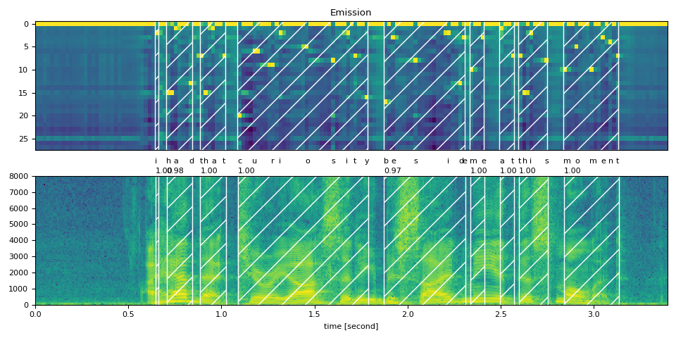
可视化
现在让我们看一下对齐结果,并将原始语音分割成单词。
def plot_alignments(waveform, token_spans, emission, transcript, sample_rate=bundle.sample_rate):
    ratio = waveform.size(1) / emission.size(1) / sample_rate

    fig, axes = plt.subplots(2, 1)
    axes[0].imshow(emission[0].detach().cpu().T, aspect="auto")
    axes[0].set_title("Emission")
    axes[0].set_xticks([])

    axes[1].specgram(waveform[0], Fs=sample_rate)
    for t_spans, chars in zip(token_spans, transcript):
        t0, t1 = t_spans[0].start + 0.1, t_spans[-1].end - 0.1
        axes[0].axvspan(t0 - 0.5, t1 - 0.5, facecolor="None", hatch="/", edgecolor="white")
        axes[1].axvspan(ratio * t0, ratio * t1, facecolor="None", hatch="/", edgecolor="white")
        axes[1].annotate(f"{_score(t_spans):.2f}", (ratio * t0, sample_rate * 0.51), annotation_clip=False)

        for span, char in zip(t_spans, chars):
            t0 = span.start * ratio
            axes[1].annotate(char, (t0, sample_rate * 0.55), annotation_clip=False)

    axes[1].set_xlabel("time [second]")
    axes[1].set_xlim([0, None])
    fig.tight_layout()
plot_alignments(waveform, word_spans, emission, TRANSCRIPT)
对 blank 个标记的处理不一致
当将标记级别的对齐拆分为单词时,你会发现一些空白标记的处理方式不同,这使得结果的解释变得有些模糊。
当我们绘制这些得分时,这一点很容易看出。下图显示了单词区域和非单词区域,以及非空白标记的帧级得分。
def plot_scores(word_spans, scores):
    fig, ax = plt.subplots()
    span_xs, span_hs = [], []
    ax.axvspan(word_spans[0][0].start - 0.05, word_spans[-1][-1].end + 0.05, facecolor="paleturquoise", edgecolor="none", zorder=-1)
    for t_span in word_spans:
        for span in t_span:
            for t in range(span.start, span.end):
                span_xs.append(t + 0.5)
                span_hs.append(scores[t].item())
            ax.annotate(LABELS[span.token], (span.start, -0.07))
        ax.axvspan(t_span[0].start - 0.05, t_span[-1].end + 0.05, facecolor="mistyrose", edgecolor="none", zorder=-1)
    ax.bar(span_xs, span_hs, color="lightsalmon", edgecolor="coral")
    ax.set_title("Frame-level scores and word segments")
    ax.set_ylim(-0.1, None)
    ax.grid(True, axis="y")
    ax.axhline(0, color="black")
    fig.tight_layout()


plot_scores(word_spans, alignment_scores)
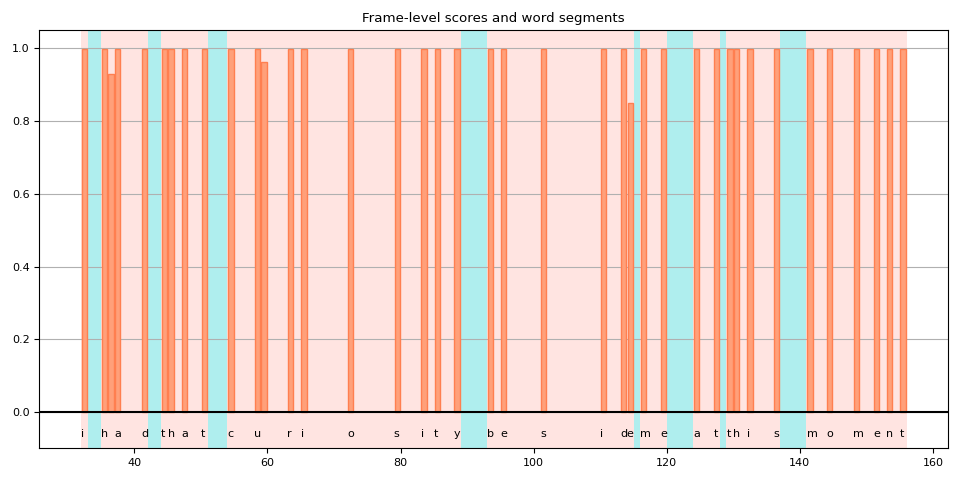
在这张图中,空白标记是那些没有垂直条的高亮区域。 你可以看到有一些空白标记被解释为单词的一部分(用红色高亮显示),而其他空白标记(用蓝色高亮显示)则不是。
原因之一是模型在训练时没有使用词边界标签。空白标记不仅被视为重复,还被视为词与词之间的静音部分。
但随后,一个问题出现了。单词结束或接近结束后的帧应该是静音还是重复?
在上面的例子中,如果你回到之前绘制的频谱图和词区域图,你会发现“curiosity”中的“y”之后,仍然有一些频率桶中的活动。
如果该帧包含在单词中,是否更准确?
不幸的是,CTC 并未提供对这一问题的全面解决方案。 使用 CTC 训练的模型已知会表现出“尖峰”响应, 也就是说,它们倾向于在标签出现时产生一个尖峰,但该尖峰不会持续整个标签的时长。 (注意:预训练的 Wav2Vec2 模型往往在标签出现的开始处产生尖峰,但这并非总是如此。)
[Zeyer et al., 2021] 对 CTC 的峰值行为进行了深入分析。 我们鼓励有兴趣了解更多的人参考该论文。 以下是论文中的一段引文,正是我们在这里面临的问题。
Peaky behavior can be problematic in certain cases, e.g. when an application requires to not use the blank label, e.g. to get meaningful time accurate alignments of phonemes to a transcription.
高级:处理包含 <star> 个标记的转录文本
现在让我们看看当转录文本部分缺失时,如何利用能够模拟任何标记的<star>标记来提高对齐质量。
此处我们使用与上文相同的英文示例。但我们从转录文本中去除了开头的文本 “i had that curiosity beside me at”。
将音频与这样的转录文本对齐会导致现有单词“this”的对齐出现错误。然而,可以通过使用
<star> 标记来建模缺失的文本来缓解此问题。
首先,我们扩展字典以包含 <star> 个标记。
DICTIONARY["*"] = len(DICTIONARY)
接下来,我们通过添加一个额外的维度来扩展发射张量,该维度对应于<star>标记。
star_dim = torch.zeros((1, emission.size(1), 1), device=emission.device, dtype=emission.dtype)
emission = torch.cat((emission, star_dim), 2)

assert len(DICTIONARY) == emission.shape[2]

plot_emission(emission[0])

以下函数将所有过程结合起来,并一次性从发射中计算出词段。
def compute_alignments(emission, transcript, dictionary):
    tokens = [dictionary[char] for word in transcript for char in word]
    alignment, scores = align(emission, tokens)
    token_spans = F.merge_tokens(alignment, scores)
    word_spans = unflatten(token_spans, [len(word) for word in transcript])
    return word_spans
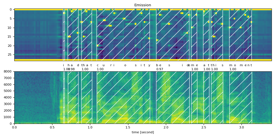
完整文本
word_spans = compute_alignments(emission, TRANSCRIPT, DICTIONARY)
plot_alignments(waveform, word_spans, emission, TRANSCRIPT)
部分转录文本,包含 <star> 个标记
现在我们将转录文本的第一部分替换为 <star> 个标记。
transcript = "* this moment".split()
word_spans = compute_alignments(emission, transcript, DICTIONARY)
plot_alignments(waveform, word_spans, emission, transcript)
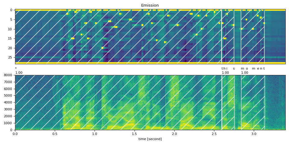
preview_word(waveform, word_spans[0], num_frames, transcript[0])
* (1.00): 0.000 - 2.595 sec
preview_word(waveform, word_spans[1], num_frames, transcript[1])
this (1.00): 2.595 - 2.756 sec
preview_word(waveform, word_spans[2], num_frames, transcript[2])
moment (1.00): 2.837 - 3.138 sec
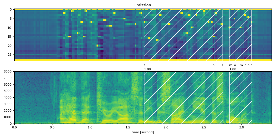
Partial Transcript without <star> token
作为对比,以下是在不使用 <star> 个标记的情况下对部分转录内容进行对齐。
它展示了使用 <star> 个标记处理删除错误的效果。
transcript = "this moment".split()
word_spans = compute_alignments(emission, transcript, DICTIONARY)
plot_alignments(waveform, word_spans, emission, transcript)
结论
在本教程中,我们介绍了如何使用 torchaudio 的强制对齐 API 来对齐和分割语音文件,并演示了一个高级用法:当存在转录错误时,引入一个 <star> 个标记如何提高对齐准确性。
致谢
感谢 Vineel Pratap 和 Zhaoheng Ni 开发并开源了强制对齐 API。
脚本的总运行时间: ( 0 分钟 35.903 秒)