注意

转到末尾以下载完整示例代码。

循环DQN：训练循环策略¶

作者: Vincent Moens

你将学到什么

如何在 TorchRL 中的演员中加入 RNN
如何使用基于内存的策略与重放缓冲区和损失模块

先决条件

PyTorch v2.0.0
gym[mujoco]
进度条

概览¶

基于记忆的策略不仅在观测信息部分可观测时至关重要，而且在必须考虑时间维度以做出明智决策时也同样重要。

循环神经网络长期以来一直是基于记忆的策略的常用工具。其基本思想是在连续两个时间步之间于内存中维持一个循环状态，并将该状态与当前观测值一同作为策略的输入。

本教程展示了如何使用 TorchRL 在策略中集成 RNN。

核心收获：

在 TorchRL 中将 RNN 集成到演员中；
使用基于内存的策略，配合重放缓冲区和损失模块。

在 TorchRL 中使用 RNN 的核心思想是利用 TensorDict 作为数据载体，在各个时间步之间传递隐藏状态。我们将构建一个策略，该策略从当前的 TensorDict 中读取上一时刻的循环状态，并将当前的循环状态写入下一时刻状态对应的 TensorDict 中：

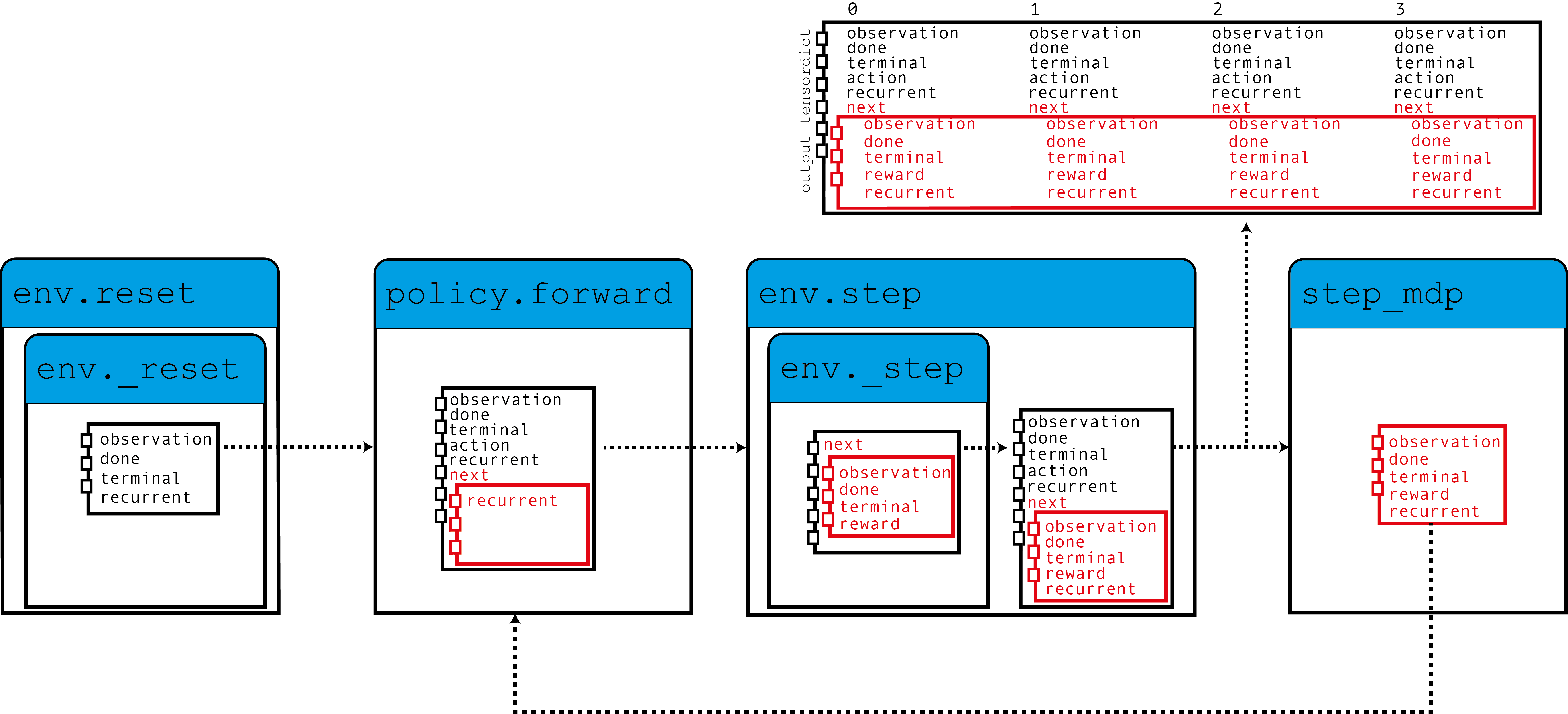
如图所示，我们的环境将零初始化的循环状态填充到TensorDict中，这些循环状态与观察值一起被策略读取以生成动作，并且这些循环状态将在下一步使用。当调用step_mdp()函数时，来自下一个状态的循环状态被带入当前的TensorDict。让我们看看这在实践中是如何实现的。

如果您在 Google Colab 中运行此代码，请确保安装以下依赖项：

!pip3 install torchrl
!pip3 install gym[mujoco]
!pip3 install tqdm

设置¶

import torch
import tqdm
from tensordict.nn import (
    TensorDictModule as Mod,
    TensorDictSequential,
    TensorDictSequential as Seq,
)
from torch import nn
from torchrl.collectors import SyncDataCollector
from torchrl.data import LazyMemmapStorage, TensorDictReplayBuffer
from torchrl.envs import (
    Compose,
    ExplorationType,
    GrayScale,
    InitTracker,
    ObservationNorm,
    Resize,
    RewardScaling,
    set_exploration_type,
    StepCounter,
    ToTensorImage,
    TransformedEnv,
)
from torchrl.envs.libs.gym import GymEnv
from torchrl.modules import ConvNet, EGreedyModule, LSTMModule, MLP, QValueModule
from torchrl.objectives import DQNLoss, SoftUpdate

is_fork = multiprocessing.get_start_method() == "fork"
device = (
    torch.device(0)
    if torch.cuda.is_available() and not is_fork
    else torch.device("cpu")
)

环境¶

和往常一样，第一步是构建我们的环境：这有助于我们定义问题，并据此构建策略网络。在本教程中，我们将运行一个基于像素的单实例 CartPole Gym 环境，并应用一些自定义变换：转为灰度图、调整尺寸至 84×84、缩小奖励值，并对观测值进行归一化处理。

注意

The StepCounter 变换是辅助的。由于CartPole任务的目标是使轨迹尽可能长，计数步骤可以帮助我们跟踪策略的表现。

对于本教程的目的，有两个变换非常重要：

InitTracker 将在调用 reset() 时添加一个 "is_init" 布尔掩码到 TensorDict 中，以跟踪哪些步骤需要重置 RNN 隐藏状态。
The TensorDictPrimer 转换稍微复杂一些。它不是使用RNN策略所必需的。但是，它指示环境（随后是收集器）期望一些额外的键。一旦添加，调用 env.reset() 将使用零张量填充引物中指示的条目。由于策略期望这些张量，收集器将在收集过程中传递它们。最终，我们将把隐藏状态存储在重放缓冲区中，这将帮助我们在损失模块中引导RNN操作的计算（否则将从0开始）。总之：不包括这个转换不会对我们的策略训练产生太大影响，但它会使收集的数据和重放缓冲区中的循环键消失，从而导致稍欠优化的训练。幸运的是，我们提出的 LSTMModule 配备了一个辅助方法来构建这样的转换，因此我们可以等到构建它！

env = TransformedEnv(
    GymEnv("CartPole-v1", from_pixels=True, device=device),
    Compose(
        ToTensorImage(),
        GrayScale(),
        Resize(84, 84),
        StepCounter(),
        InitTracker(),
        RewardScaling(loc=0.0, scale=0.1),
        ObservationNorm(standard_normal=True, in_keys=["pixels"]),
    ),
)

一如既往，我们需要手动初始化我们的归一化常数：

env.transform[-1].init_stats(1000, reduce_dim=[0, 1, 2], cat_dim=0, keep_dims=[0])
td = env.reset()

政策¶

我们的策略将包含3个组件：一个ConvNet主干，一个LSTMModule记忆层和一个浅层的MLP块，该块将LSTM输出映射到动作值。

卷积网络¶

我们构建了一个带有 torch.nn.AdaptiveAvgPool2d 的卷积网络，它将输出压缩为大小为64的向量。ConvNet 可以帮助我们实现这一点：

feature = Mod(
    ConvNet(
        num_cells=[32, 32, 64],
        squeeze_output=True,
        aggregator_class=nn.AdaptiveAvgPool2d,
        aggregator_kwargs={"output_size": (1, 1)},
        device=device,
    ),
    in_keys=["pixels"],
    out_keys=["embed"],
)

我们对一批数据执行第一个模块，以获取输出向量的尺寸：

n_cells = feature(env.reset())["embed"].shape[-1]

LSTM 模块¶

TorchRL 提供了一个专门的 LSTMModule 类来在您的代码库中集成 LSTMs。它是一个 TensorDictModuleBase 子类：因此，它有一组 in_keys 和 out_keys 来指示在模块执行期间应该读取和写入/更新哪些值。该类附带了这些属性的可自定义预定义值，以方便其构建。

注意

使用限制: 该类支持几乎所有LSTM功能，例如 dropout 或多层LSTM。但是，为了遵循TorchRL的约定，此LSTM必须将 batch_first 属性设置为 True，这在PyTorch中不是默认值。但是，我们的 LSTMModule 改变了这种默认行为，因此我们可以直接调用。

此外，LSTM 不能将 bidirectional 属性设置为 True，因为这在在线环境中无法使用。在这种情况下，默认值是正确的。

lstm = LSTMModule(
    input_size=n_cells,
    hidden_size=128,
    device=device,
    in_key="embed",
    out_key="embed",
)

让我们来看看 LSTM Module 类，特别是它的 in 和 out_keys：

print("in_keys", lstm.in_keys)
print("out_keys", lstm.out_keys)

in_keys ['embed', 'recurrent_state_h', 'recurrent_state_c', 'is_init']
out_keys ['embed', ('next', 'recurrent_state_h'), ('next', 'recurrent_state_c')]

我们可以看到这些值包含了我们指定为 in_key（和 out_key）的键，以及循环键名。out_keys 以“next”前缀开头，表示它们需要写入“next”TensorDict 中。我们使用这种约定（可以通过传递 in_keys/out_keys 参数来覆盖），以确保调用 step_mdp() 将会将循环状态移动到根 TensorDict 中，使其在下一次调用时可供 RNN 使用（参见介绍中的图示）。

如前所述，我们还有一个可选的转换需要添加到我们的环境中，以确保循环状态被传递到缓冲区。make_tensordict_primer()方法正好做到了这一点：

env.append_transform(lstm.make_tensordict_primer())

TransformedEnv(
    env=GymEnv(env=CartPole-v1, batch_size=torch.Size([]), device=cpu),
    transform=Compose(
            ToTensorImage(keys=['pixels']),
            GrayScale(keys=['pixels']),
            Resize(w=84, h=84, interpolation=InterpolationMode.BILINEAR, keys=['pixels']),
            StepCounter(keys=[]),
            InitTracker(keys=[]),
            RewardScaling(loc=0.0000, scale=0.1000, keys=['reward']),
            ObservationNorm(keys=['pixels']),
            TensorDictPrimer(primers=Composite(
                recurrent_state_h: UnboundedContinuous(
                    shape=torch.Size([1, 128]),
                    space=ContinuousBox(
                        low=Tensor(shape=torch.Size([1, 128]), device=cpu, dtype=torch.float32, contiguous=True),
                        high=Tensor(shape=torch.Size([1, 128]), device=cpu, dtype=torch.float32, contiguous=True)),
                    device=cpu,
                    dtype=torch.float32,
                    domain=continuous),
                recurrent_state_c: UnboundedContinuous(
                    shape=torch.Size([1, 128]),
                    space=ContinuousBox(
                        low=Tensor(shape=torch.Size([1, 128]), device=cpu, dtype=torch.float32, contiguous=True),
                        high=Tensor(shape=torch.Size([1, 128]), device=cpu, dtype=torch.float32, contiguous=True)),
                    device=cpu,
                    dtype=torch.float32,
                    domain=continuous),
                device=cpu,
                shape=torch.Size([])), default_value={'recurrent_state_h': 0.0, 'recurrent_state_c': 0.0}, random=None)))

就这样！我们可以打印环境信息，以确认在添加了入门指南后，一切看起来都正常。

print(env)

TransformedEnv(
    env=GymEnv(env=CartPole-v1, batch_size=torch.Size([]), device=cpu),
    transform=Compose(
            ToTensorImage(keys=['pixels']),
            GrayScale(keys=['pixels']),
            Resize(w=84, h=84, interpolation=InterpolationMode.BILINEAR, keys=['pixels']),
            StepCounter(keys=[]),
            InitTracker(keys=[]),
            RewardScaling(loc=0.0000, scale=0.1000, keys=['reward']),
            ObservationNorm(keys=['pixels']),
            TensorDictPrimer(primers=Composite(
                recurrent_state_h: UnboundedContinuous(
                    shape=torch.Size([1, 128]),
                    space=ContinuousBox(
                        low=Tensor(shape=torch.Size([1, 128]), device=cpu, dtype=torch.float32, contiguous=True),
                        high=Tensor(shape=torch.Size([1, 128]), device=cpu, dtype=torch.float32, contiguous=True)),
                    device=cpu,
                    dtype=torch.float32,
                    domain=continuous),
                recurrent_state_c: UnboundedContinuous(
                    shape=torch.Size([1, 128]),
                    space=ContinuousBox(
                        low=Tensor(shape=torch.Size([1, 128]), device=cpu, dtype=torch.float32, contiguous=True),
                        high=Tensor(shape=torch.Size([1, 128]), device=cpu, dtype=torch.float32, contiguous=True)),
                    device=cpu,
                    dtype=torch.float32,
                    domain=continuous),
                device=cpu,
                shape=torch.Size([])), default_value={'recurrent_state_h': 0.0, 'recurrent_state_c': 0.0}, random=None)))

MLP¶

我们使用单层多层感知机（MLP）来表示将用于策略的动作值。

mlp = MLP(
    out_features=2,
    num_cells=[
        64,
    ],
    device=device,
)

并将偏差填充为零：

mlp[-1].bias.data.fill_(0.0)
mlp = Mod(mlp, in_keys=["embed"], out_keys=["action_value"])

使用Q值选择动作¶

我们策略的最后一部分是Q值模块。 Q值模块 QValueModule 将读取由我们的MLP生成的"action_values"键，并从中收集具有最大值的动作。我们需要做的唯一一件事是指定动作空间，这可以通过传递字符串或动作规范来完成。这允许我们使用分类（有时称为“稀疏”）编码或其独热版本。

qval = QValueModule(action_space=None, spec=env.action_spec)

注意

TorchRL 还提供了一个包装类 torchrl.modules.QValueActor，该类将一个模块与一个 QValueModule 一起包装在一个 Sequential 中，就像我们在这里显式地做的那样。这样做几乎没有优势，并且过程不够透明，但最终结果将类似于我们在这里所做的。

我们现在可以将这些内容组合在一起了 TensorDictSequential

stoch_policy = Seq(feature, lstm, mlp, qval)

DQN作为一种确定性算法，探索是其重要组成部分。我们将使用一个\(\epsilon\)-贪婪策略，epsilon为0.2，并逐渐衰减至0。这种衰减是通过调用step()实现的（参见下面的训练循环）。

exploration_module = EGreedyModule(
    annealing_num_steps=1_000_000, spec=env.action_spec, eps_init=0.2
)
stoch_policy = TensorDictSequential(
    stoch_policy,
    exploration_module,
)

使用模型进行损失计算¶

我们构建的模型非常适合在序列环境中使用。然而，类 torch.nn.LSTM 可以使用 cuDNN 优化的后端在 GPU 设备上更快地运行 RNN 序列。我们不想错过这样一个加快训练循环的机会！要使用它，我们只需要告诉 LSTM 模块在“循环模式”下运行当被损失函数使用时。由于我们通常希望有两个 LSTM 模块的副本，我们通过调用一个 set_recurrent_mode() 方法来实现这一点，该方法将返回一个新的 LSTM 实例（具有共享权重），该实例将假设输入数据是按顺序排列的。

policy = Seq(feature, lstm.set_recurrent_mode(True), mlp, qval)

因为我们仍有几个未初始化的参数，所以在创建优化器等之前，应先对它们进行初始化。

policy(env.reset())

TensorDict(
    fields={
        action: Tensor(shape=torch.Size([2]), device=cpu, dtype=torch.int64, is_shared=False),
        action_value: Tensor(shape=torch.Size([2]), device=cpu, dtype=torch.float32, is_shared=False),
        chosen_action_value: Tensor(shape=torch.Size([1]), device=cpu, dtype=torch.float32, is_shared=False),
        done: Tensor(shape=torch.Size([1]), device=cpu, dtype=torch.bool, is_shared=False),
        embed: Tensor(shape=torch.Size([128]), device=cpu, dtype=torch.float32, is_shared=False),
        is_init: Tensor(shape=torch.Size([1]), device=cpu, dtype=torch.bool, is_shared=False),
        next: TensorDict(
            fields={
                recurrent_state_c: Tensor(shape=torch.Size([1, 128]), device=cpu, dtype=torch.float32, is_shared=False),
                recurrent_state_h: Tensor(shape=torch.Size([1, 128]), device=cpu, dtype=torch.float32, is_shared=False)},
            batch_size=torch.Size([]),
            device=cpu,
            is_shared=False),
        pixels: Tensor(shape=torch.Size([1, 84, 84]), device=cpu, dtype=torch.float32, is_shared=False),
        recurrent_state_c: Tensor(shape=torch.Size([1, 128]), device=cpu, dtype=torch.float32, is_shared=False),
        recurrent_state_h: Tensor(shape=torch.Size([1, 128]), device=cpu, dtype=torch.float32, is_shared=False),
        step_count: Tensor(shape=torch.Size([1]), device=cpu, dtype=torch.int64, is_shared=False),
        terminated: Tensor(shape=torch.Size([1]), device=cpu, dtype=torch.bool, is_shared=False),
        truncated: Tensor(shape=torch.Size([1]), device=cpu, dtype=torch.bool, is_shared=False)},
    batch_size=torch.Size([]),
    device=cpu,
    is_shared=False)

DQN 损失¶

Out DQN loss 需要我们传递策略和，再次，动作空间。虽然这可能看起来冗余，但这是很重要的，因为我们希望确保 DQNLoss 和 QValueModule 类是兼容的，但彼此之间没有强依赖关系。

要使用Double-DQN，我们需要一个delay_value参数，该参数将创建网络参数的非可微副本，用于作为目标网络。

loss_fn = DQNLoss(policy, action_space=env.action_spec, delay_value=True)

由于我们使用的是双DQN，我们需要更新目标参数。我们将使用一个 SoftUpdate 实例来执行这项工作。

updater = SoftUpdate(loss_fn, eps=0.95)

optim = torch.optim.Adam(policy.parameters(), lr=3e-4)

Collector 和重放缓冲区¶

我们构建了最简单的数据收集器。我们将尝试用一百万帧来训练我们的算法，每次扩展缓冲区50帧。缓冲区将被设计为存储2万个轨迹，每个轨迹包含50个步骤。在每次优化步骤（每收集一次数据有16个优化步骤）中，我们将从缓冲区中收集4个项目，总共200个转换。我们将使用一个LazyMemmapStorage 存储来将数据保存在磁盘上。

注意

为提高效率，此处仅运行数千次迭代。在实际应用中，总帧数应设为 100 万。

collector = SyncDataCollector(env, stoch_policy, frames_per_batch=50, total_frames=200)
rb = TensorDictReplayBuffer(
    storage=LazyMemmapStorage(20_000), batch_size=4, prefetch=10
)

训练循环¶

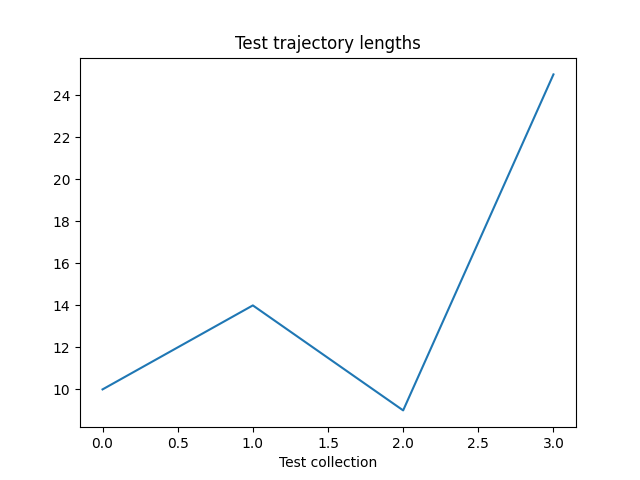
为跟踪训练进度，我们将每收集 50 次数据后在环境中运行一次策略，并在训练完成后绘制结果。

utd = 16
pbar = tqdm.tqdm(total=collector.total_frames)
longest = 0

traj_lens = []
for i, data in enumerate(collector):
    if i == 0:
        print(
            "Let us print the first batch of data.\nPay attention to the key names "
            "which will reflect what can be found in this data structure, in particular: "
            "the output of the QValueModule (action_values, action and chosen_action_value),"
            "the 'is_init' key that will tell us if a step is initial or not, and the "
            "recurrent_state keys.\n",
            data,
        )
    pbar.update(data.numel())
    # it is important to pass data that is not flattened
    rb.extend(data.unsqueeze(0).to_tensordict().cpu())
    for _ in range(utd):
        s = rb.sample().to(device, non_blocking=True)
        loss_vals = loss_fn(s)
        loss_vals["loss"].backward()
        optim.step()
        optim.zero_grad()
    longest = max(longest, data["step_count"].max().item())
    pbar.set_description(
        f"steps: {longest}, loss_val: {loss_vals['loss'].item(): 4.4f}, action_spread: {data['action'].sum(0)}"
    )
    exploration_module.step(data.numel())
    updater.step()

    with set_exploration_type(ExplorationType.DETERMINISTIC), torch.no_grad():
        rollout = env.rollout(10000, stoch_policy)
        traj_lens.append(rollout.get(("next", "step_count")).max().item())

  0%|          | 0/200 [00:00<?, ?it/s]Let us print the first batch of data.
Pay attention to the key names which will reflect what can be found in this data structure, in particular: the output of the QValueModule (action_values, action and chosen_action_value),the 'is_init' key that will tell us if a step is initial or not, and the recurrent_state keys.
 TensorDict(
    fields={
        action: Tensor(shape=torch.Size([50, 2]), device=cpu, dtype=torch.int64, is_shared=False),
        action_value: Tensor(shape=torch.Size([50, 2]), device=cpu, dtype=torch.float32, is_shared=False),
        chosen_action_value: Tensor(shape=torch.Size([50, 1]), device=cpu, dtype=torch.float32, is_shared=False),
        collector: TensorDict(
            fields={
                traj_ids: Tensor(shape=torch.Size([50]), device=cpu, dtype=torch.int64, is_shared=False)},
            batch_size=torch.Size([50]),
            device=None,
            is_shared=False),
        done: Tensor(shape=torch.Size([50, 1]), device=cpu, dtype=torch.bool, is_shared=False),
        embed: Tensor(shape=torch.Size([50, 128]), device=cpu, dtype=torch.float32, is_shared=False),
        is_init: Tensor(shape=torch.Size([50, 1]), device=cpu, dtype=torch.bool, is_shared=False),
        next: TensorDict(
            fields={
                done: Tensor(shape=torch.Size([50, 1]), device=cpu, dtype=torch.bool, is_shared=False),
                is_init: Tensor(shape=torch.Size([50, 1]), device=cpu, dtype=torch.bool, is_shared=False),
                pixels: Tensor(shape=torch.Size([50, 1, 84, 84]), device=cpu, dtype=torch.float32, is_shared=False),
                recurrent_state_c: Tensor(shape=torch.Size([50, 1, 128]), device=cpu, dtype=torch.float32, is_shared=False),
                recurrent_state_h: Tensor(shape=torch.Size([50, 1, 128]), device=cpu, dtype=torch.float32, is_shared=False),
                reward: Tensor(shape=torch.Size([50, 1]), device=cpu, dtype=torch.float32, is_shared=False),
                step_count: Tensor(shape=torch.Size([50, 1]), device=cpu, dtype=torch.int64, is_shared=False),
                terminated: Tensor(shape=torch.Size([50, 1]), device=cpu, dtype=torch.bool, is_shared=False),
                truncated: Tensor(shape=torch.Size([50, 1]), device=cpu, dtype=torch.bool, is_shared=False)},
            batch_size=torch.Size([50]),
            device=None,
            is_shared=False),
        pixels: Tensor(shape=torch.Size([50, 1, 84, 84]), device=cpu, dtype=torch.float32, is_shared=False),
        recurrent_state_c: Tensor(shape=torch.Size([50, 1, 128]), device=cpu, dtype=torch.float32, is_shared=False),
        recurrent_state_h: Tensor(shape=torch.Size([50, 1, 128]), device=cpu, dtype=torch.float32, is_shared=False),
        step_count: Tensor(shape=torch.Size([50, 1]), device=cpu, dtype=torch.int64, is_shared=False),
        terminated: Tensor(shape=torch.Size([50, 1]), device=cpu, dtype=torch.bool, is_shared=False),
        truncated: Tensor(shape=torch.Size([50, 1]), device=cpu, dtype=torch.bool, is_shared=False)},
    batch_size=torch.Size([50]),
    device=None,
    is_shared=False)

 25%|██▌       | 50/200 [00:00<00:01, 130.78it/s]
 25%|██▌       | 50/200 [00:11<00:01, 130.78it/s]
steps: 9, loss_val:  0.0006, action_spread: tensor([46,  4]):  25%|██▌       | 50/200 [00:31<00:01, 130.78it/s]
steps: 9, loss_val:  0.0006, action_spread: tensor([46,  4]):  50%|█████     | 100/200 [00:32<00:37,  2.64it/s]
steps: 11, loss_val:  0.0004, action_spread: tensor([44,  6]):  50%|█████     | 100/200 [01:03<00:37,  2.64it/s]
steps: 11, loss_val:  0.0004, action_spread: tensor([44,  6]):  75%|███████▌  | 150/200 [01:04<00:24,  2.01it/s]
steps: 17, loss_val:  0.0004, action_spread: tensor([12, 38]):  75%|███████▌  | 150/200 [01:35<00:24,  2.01it/s]
steps: 17, loss_val:  0.0004, action_spread: tensor([12, 38]): 100%|██████████| 200/200 [01:35<00:00,  1.81it/s]
steps: 17, loss_val:  0.0003, action_spread: tensor([43,  7]): 100%|██████████| 200/200 [02:07<00:00,  1.81it/s]

让我们绘制我们的结果：

if traj_lens:
    from matplotlib import pyplot as plt

    plt.plot(traj_lens)
    plt.xlabel("Test collection")
    plt.title("Test trajectory lengths")

结论¶

我们已经了解了如何在 TorchRL 的策略中整合 RNN。你现在应该能够：

创建一个充当TensorDictModule的LSTM模块
向LSTM模块指示需要重置通过一个 InitTracker 转换
将此模块集成到策略中和损失模块中
确保采集器知晓循环状态条目，以便它们能与其余数据一同存储在回放缓冲区中

进一步阅读¶

TorchRL 文档可在此处找到此处。

脚本总运行时间： (3 分钟 8.564 秒)

估计内存使用量： 2233 MB

通过 Sphinx-Gallery 生成的画廊